A year ago I submitted the paper Topology-guided accelerated vector field streamline visualization to The Visual Computer, which has since been accepted. My paper is now available online here. Please don’t use LibGen or Sci-Hub to download my paper, cuz that would be naughty :)

Before we begin, massive thanks to Marek Fiser’s blog post and Yilun Yang’s previous work, both of which I drew inspiration (and code) from, without which this paper wouldn’t have been possible.

Abstract

In the paper, I proposed an adaptive method for locating planar critical points during streamline and streamtube tracings. New seed points are dynamically added on-the-fly and traced iteratively. See it work in action here:

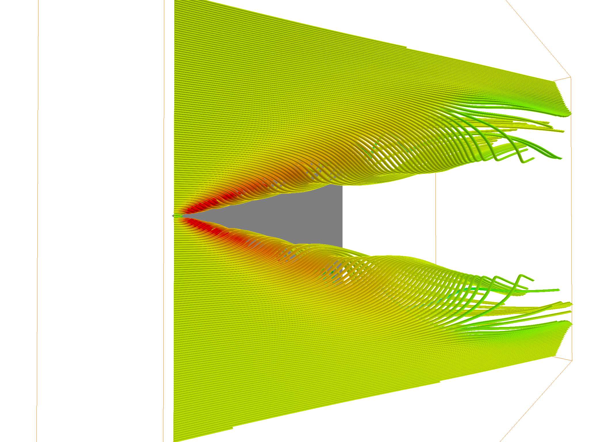
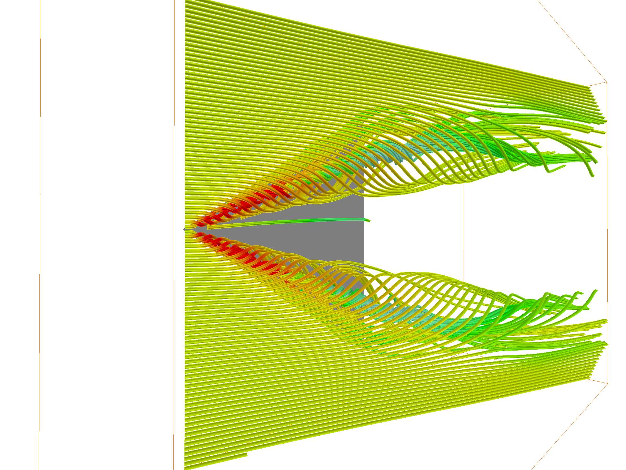
Notice anything different? The left one is uniformly seeded, and the right one is seeded with the adaptive planar critical point method. Compared to the left one, our method dynamically spawns new seed points when critical points were discovered, where the vector field has the most significant changes. This results in much richer streamlines and streamtubes, capable of producing more information with the same amount of seed points. For example, more streamlines trace the turbulence underneath the upper drafts.

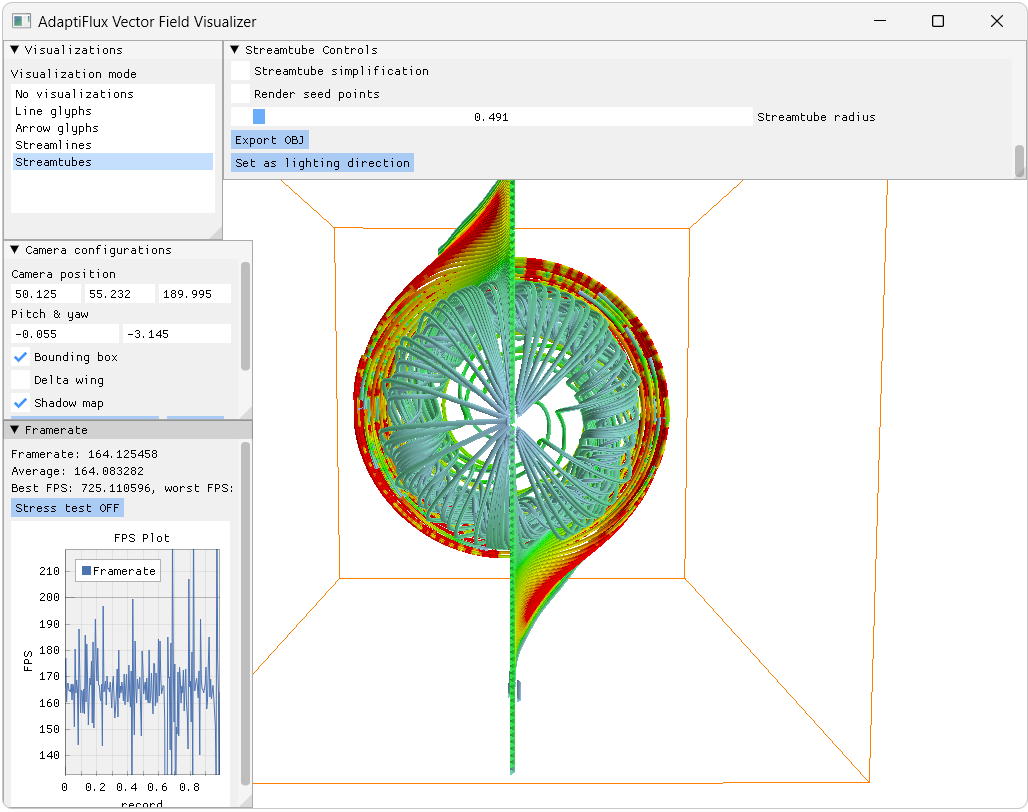
We also made a complete vector field visualization system for this, called AdaptiFlux. It supports various vector field visualization modes, including lines, arrow glyphs, streamlines and streamtubes, with our method implemented. Here’s a screenshot:

Introduction

To trace streamlines in a vector field, initial “seeds”, or “seed points”, must be specified. Those seeds are then shifted according to the underlying vector field direction and velocity, drawing out the streamlines in the process. The fancy name for the above process is called Line Integral Convolution (LIC) - because to draw the line, we have to move very little delta steps, effectively performing an integration. Think about a camera pointing at the starry night with crazy long exposure.

Since initial seeds must be provided, it’s quite easy to then know the final visualization result will be highly dependent on the seeding location. Here’s the delta wing scene visualized using two sets of initial seeds, with each of them being slightly different. This is stolen directly from Marek’s blog:

However, sometimes the streamlines traced won’t be good even with a relatively good initial streamline placement. Some important twists and turns only happens later down the line, and how can we capture that if we’ve already spent all the seeds at the beginning? And how do we even find these twists and turns, if possible?

Introducing the our adaptive seeding method. In a massive nutshell, suppose we have a seed quota of \(N = 200\). the algorithm first conserves half of them to be used later, then trace the initial 100 seeds. During the initial trace, we detect if these seeds are falling into critical points. And if they do, a seed point explosion event occurs, where new seed points are created around the critical region. Those new seed points are then traced during the second iteration, and so on. The tracing doesn’t stop until:

1. No new seed points are created during the last iteration.
2. The seed point quota is used up (that is, \(N\) seeds have already been traced.)

When Should We Explode?

How do we determine when to trigger an explosion event though? Well, we split it into two categories. First, we sample the vector field under point \(p\). If \(v(p) = 0\), that means we are approaching a 3D critical point. A simple rationale for this is that the storm is always quitest in its center. 3D critical points tend to be quite complex, with the vectors around it being possible to be pointing in all sorts of directions. Like this:

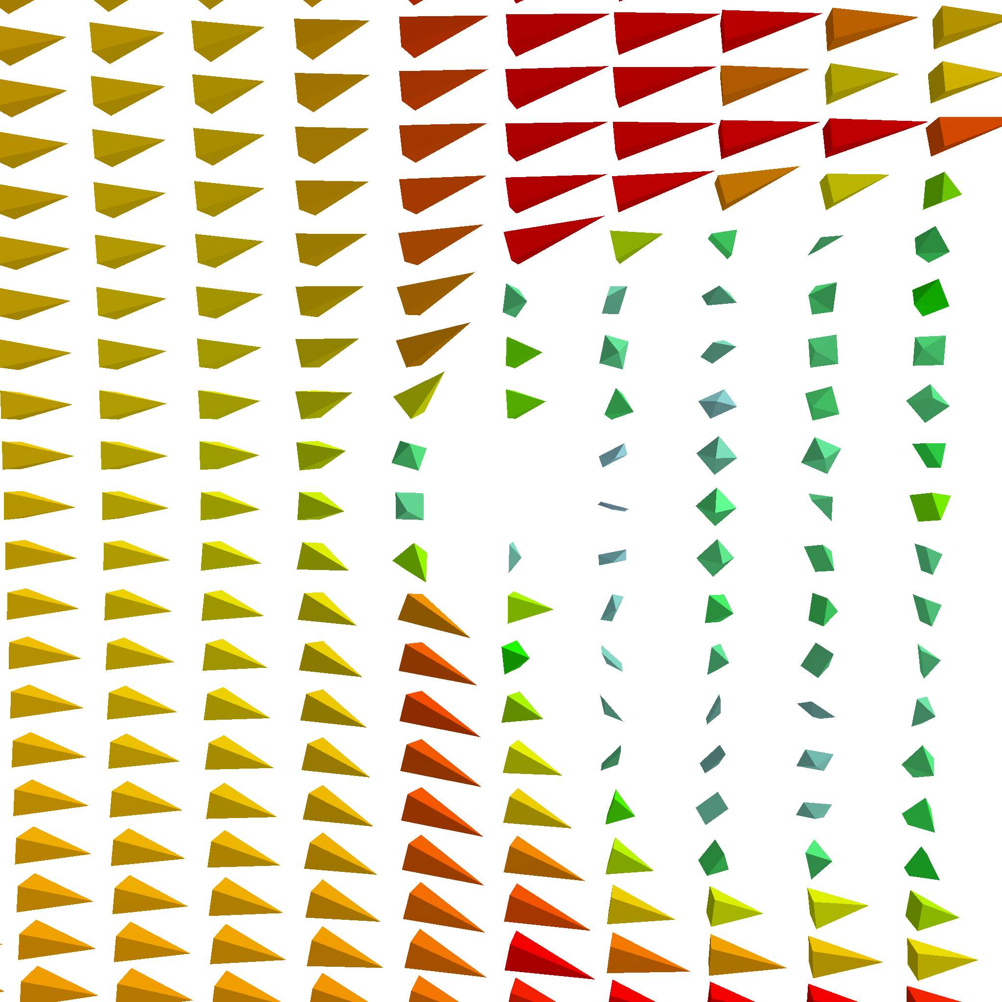
This is only a cross section of a conventional critical point. Though, we can already see its quite messy around the edges. When we encounter a 3D critical point, we just generate new seed points around the old one randomly in a uniform sphere, and hope for the best.

The second category, which is also the main contribution of our paper, is a planar critical point. In a planar critical point, \(v(p)\) is not required to be 0; au contraire, they are supposed to be non-zero vectors pointing in arbitrary direction. The catch? The vectors around point \(p\), if projected onto a plane, must satisfy (or approach) 2D critical point rules.

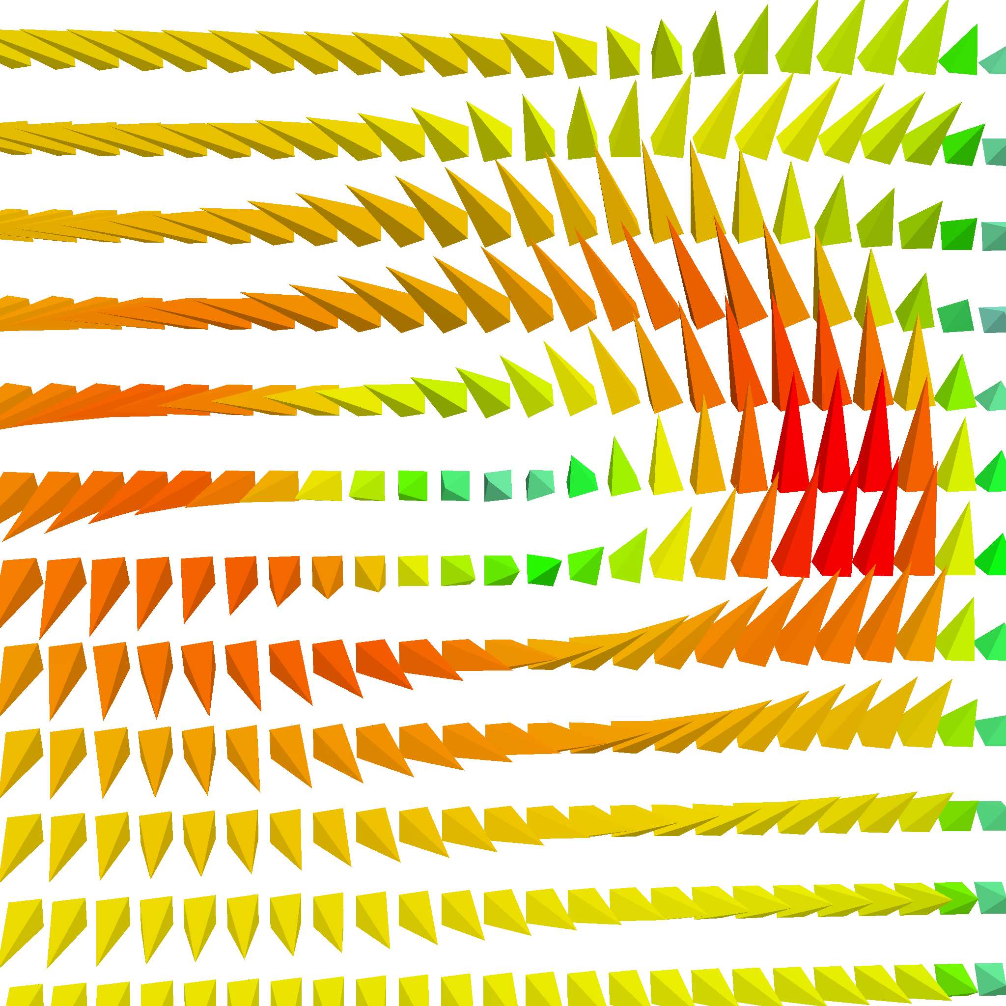
Take a look at the point in the center. Though technically not a critical point, it still kinda is because the vectors around it is…well, swirling around it. Look, finding proper words for these are hard. But hopefully, you know what I mean. This is quite useful because planar critical points can help us capture what 3D critical points can’t. Even better, we can use make use of the 2D critical point types to place new seed points so that the traced result can better reflect the critical region.

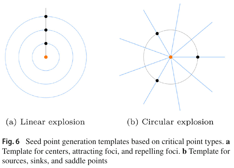
If a planar critical point type is determined to be a source, sink, or saddle point, new seed points are generated in a circular fashion; this is because circular placement can best reflect the overall topology shape of the region. In contrast, new seeds for centers, attracting foci, and repelling foci are placed in a linear fashion. This makes the most out of all the seed points, maximizing the amount of information:

How to Find Planar Critical Points?

“Well that’s good and all,” I hear you say, “but can you even locate these planar critical points guv’nor?” Well first, I haven’t heard the word “guv’nor” in ages. Second, its quite simple actually. Since planar critical points cannot be zero, it must be pointing to some sort of direction. This direction can act as a normal vector, so that the right vector r and the up vector u can be:

\[\begin{cases} r &= \frac{v(p) \times a[v(p)]}{|| v(p) \times a[v(p)] ||} \\ u &= \frac{r \times v(p)}{|| r \times v(p) ||} \end{cases}\]

Where \(a[v(p)]\) is an arbitrary up vector for \(v(p)\). Then, \(\|N\|\) neighbors are taken surrounding this plane, in a circular fashion. The sample points are quite like the “circular explosion” in the figure above:

\[N_i = p + \cos(2 \pi \frac{i - 1}{\|N\|}) r + \sin(2\pi \frac{i - 1}{\|N\|}) u\]

An alignment metric \(\mu_p\) is evalated by computing the normalized dot product of \(v(p) \text{ and } v(N_i)\):

\[\mu_p = \frac{\sum_{i=1}^{\|N\|} | \text{norm}[v(p)]^T \text{norm}[v(N_i)] |}{\|N\|}\]

If they align poorly, as in, \(\mu_p\) is under a certain threshold, then we determine that we have encountered a planar critical point. In ideal circumstances, \(\mu_p\) should equal to 0 because all its neighbors are perpendicular to \(v(p)\); but obviously this is quite difficult to happen.

In any case, once its planar critical point status was determined, we need to find out its critical point type next by finding out the eigenvalues for its 2D planar Jacobian matrix, shown in Table 1. To do this, we first find the matrix U to transform \(v(p)\) to local space (or tangent space) - so that we only have to deal with 2D vectors. That is,

\[U \frac{v(p)}{\|v(p)\|} = \begin{bmatrix}0 \\ 0\\ 1\end{bmatrix}\]

U can be solved by imaging \(v(p)\) is rotated from \(\begin{bmatrix}0 \\ 0\\ 1\end{bmatrix}\) and then reverse that rotation:

\[\begin{cases} \theta &= \arccos(v(p)_y) \\ \phi &= \begin{cases} \arccos(\frac{v(p)_z}{\sin\theta}), v(p) \geq 0 \\ \arccos(\frac{-v(p)_z}{\sin\theta}) + \pi, \text{otherwise} \end{cases} \\ U &= \begin{bmatrix} \cos\phi & \cos\theta \sin\phi & \sin\theta \cos\phi \\ 0 & -\sin\theta & \cos\theta \\ -\sin\phi \cos\theta & \cos\theta \cos\phi & \sin\theta \cos\phi \end{bmatrix}^T \end{cases}\]

We can now calculate the vector gradients along \(r\) and \(u\):

\[\begin{cases} \Delta_r v(p) &= \frac{v(p) - v(p - \varepsilon r)}{\varepsilon} \\ \Delta_u v(p) &= \frac{v(p) - v(p - \varepsilon u)}{\varepsilon} \end{cases}\]

And plug them into the Jacobian matrix:

\[J_p = \begin{bmatrix} U \Delta_r v(p)_x & U \Delta_r v(p)_y \\ U \Delta_u v(p)_x & U \Delta_u v(p)_y \\ \end{bmatrix}\]

Now that we have the Jacobian matrix, notice that sources, sinks and saddle points have real eigenvalues, while centers, attracting foci, and repelling foci do not. That means we don’t really need to find out the actual eigenvalues - we just need to find out if they have real eigenvalues. Recall that we only have two new seed placement strategies: circular, which corresponds to the former three, while linear corresponds to the latter.

With the aforementioned information, we can actually do a little trick to accelerate computation. Take a look at A quick trick for computing eigenvalues from 3Blue1Brown (and yes he’s my favorite math YouTuber) - especially around 4:28, where he showed the quick formula for finding out the eigenvalues:

\[\lambda_1, \lambda_2 = m \pm \sqrt{m^2 - p}\]

Where \(m = \frac{J_p^{1,1} + J_p^{2,2}}{2} \text{ and } p = \det(J_p)\). Notice that we can only have real roots when \(\sqrt{m^2 - p} >= 0\). This can be used to quickly determine the critical point type without ever needing to solve the eigenvalues (though, to be frank, is not that far off), and, in turn, determine the critical point type, and the seed point spawning strategy.

Stramline Simplification

After tracing the streamlines, a simple method is used to de-clutter the them - based on the global distortion value. Its just a kinda fancy name for the ratio between the actual line length and the distance between streamline starting point and ending point:

\[T(L) = \frac{\|L\|}{\|L_\text{end} - L_\text{begin}\|}\]

Streamlines are removed if \(T(L)\) is too low, or in other words, if they are too straight. Here’s how the decluttered streamlines look like. Mostly straight lines are removed to again, prioritize showing interesting streamlines first.

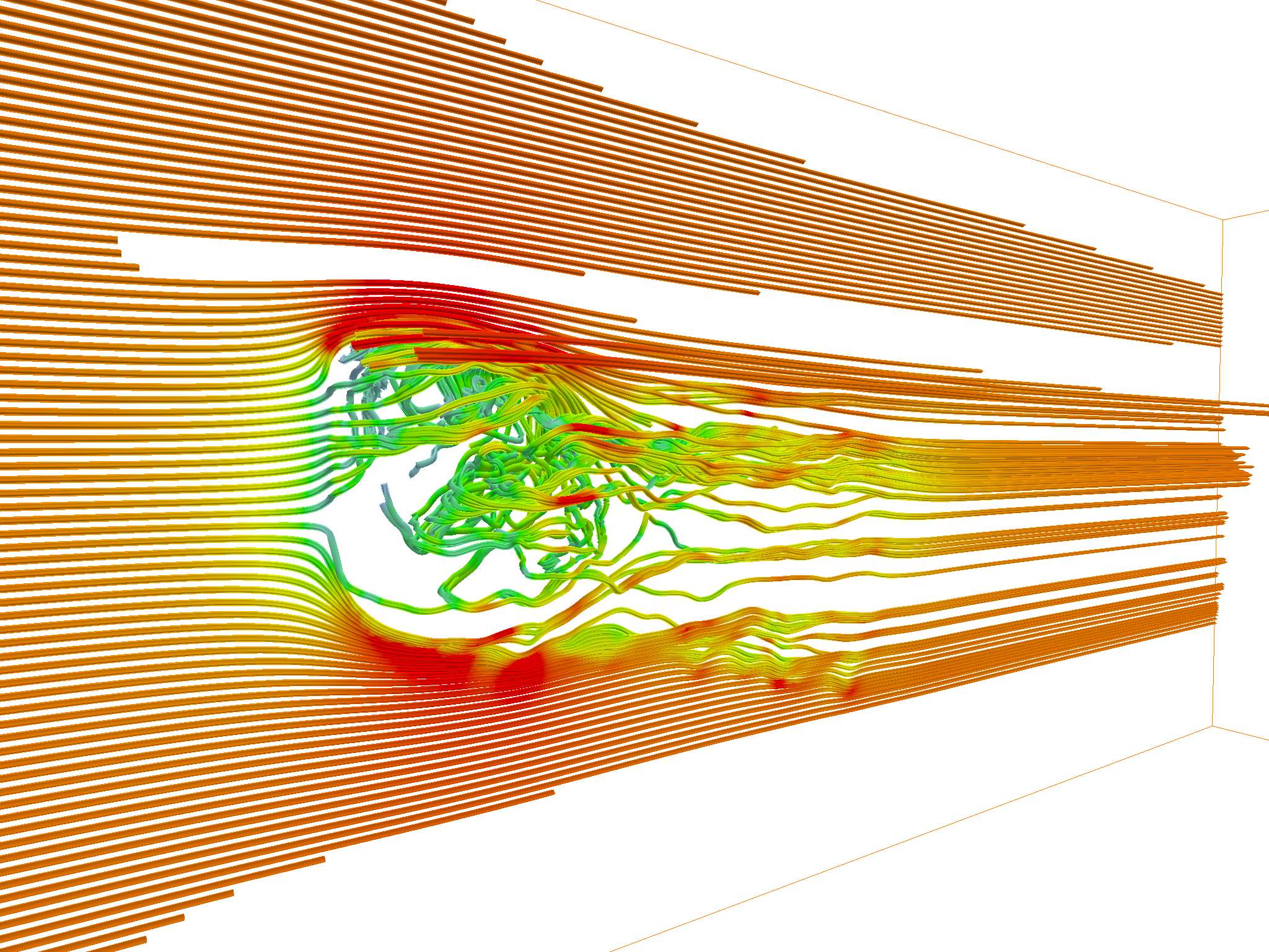
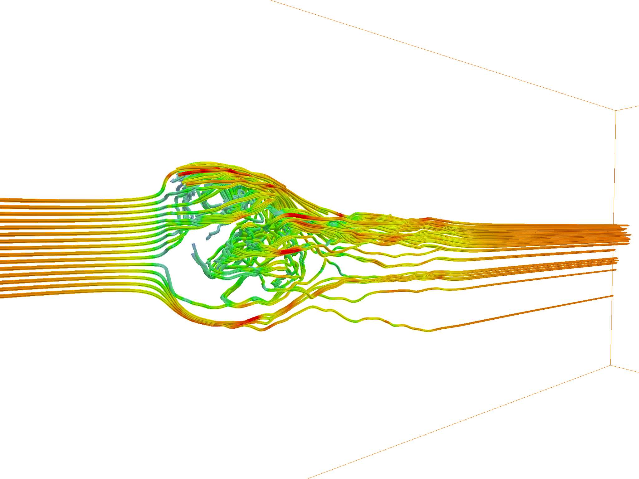
… And this is how we improve upon the original streamline tracing methods. This can be a direct plug in for other initial streamline seeding strategies as well; since our method is adaptive in nature, it could be plugged into, say, spherical seeding, and it could still be able to produce overall better streamlines. Think of it as a plug-in for the existing initial seeding strategies.

AdaptiFlux

Finally, let’s take a look at the aforementioned vector field visualization program AdaptiFlux. Because I have extended the debugger so much during the implementation it became a full-fledged CUDA-accelerated vector field visualizer. So, let’s take a look at what it’s capable of.

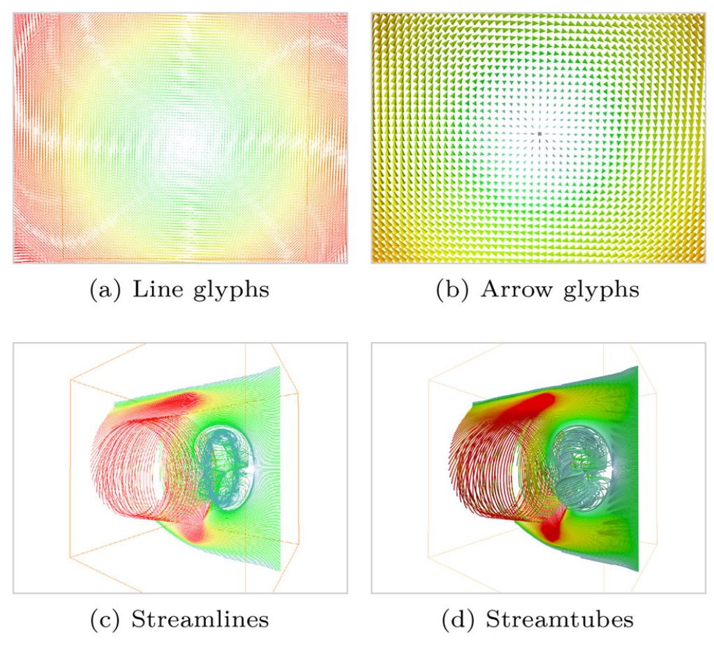
1. Four visualization methods: Lines, arrow glyphs, streamlines, and streamtubes.
2. Contains the full implementation of all proposed methods.
3. A real time FPS monitor is available right within the system.
4. Debugging features: seed point visualization visualizer, camera pose save/retrieve, and more.
5. Two initial seeding strategies: linear and spherical.
6. All visualizations are real time; tweak the parameters, and they are updated instantaneously. The rendering procedure is done by OpenGL/CUDA interoperation.

The source code of AdaptiFlux is available at https://github.com/42yeah/AdaptiFlux. Here are some extra goodies:

• Vector field datasets used in the paper.
• Uncompressed paper figures.

Conclusion

So, in conclusion, we defined a new sort of critical point in 3D, planar critical point, which we find by calculating an alignment metric around the neighbor. Once its found, the planar critical point type is determined based on the eigenvalues of the Jacobians, which we optimized a little due to the fact that we don’t actually need to evaluate the eigenvalues. The critical point type is used to determine new seed placement locations, so that we can maximize the amount of information and decrease repetitive streamlines. Finally, we made a vector field visualization system.

Obviously, quite a lot of things can be improved upon. For example, there are waaay too much parameters right now; in the future, maybe some form of machine learning can help decrease that and improve that? The implementation code quality is also something to be improved, as I was still learning CUDA as of this paper (well, actually I still am). However, seeing that I am about to graduate, I may not have time to work on this anymore (not to mention this is not a particularly good paper). So I guess there’s that.

The reason I write this blog post is because I think that accessible knowledge, not only in the form of, well, being free, but also easier to read, and therefore to learn, is important. And I always have trouble reading academic papers. That’s why I try to write a blog post on my own paper: hopefully when someone stumbles upon my paper one day, they will Google it online, and then they’ll encounter this. And hopefully the more relaxed explanation is easier to understand.

And that’s it! Whew. First blog post in 6 months! I was extremely busy the last 6 months due to school work and what not, but I am glad to be back. Stay tuned for more <3