This is a blog post from the past. Originally written at 2020-02-01.

You must’ve watched those YouTube videos, in which you can hear those sorting sounds, and those ramps getting sorted, right? If you didn’t, there’s one here. Today (or spanning multiple days for me), we are going to go over all sorts of algorithms. Bubble sort, Insertion sort, Shell sort, Merge sort, Quicksort, Heapsort, you name it. And we will start the story, with a simple dimple Bubble sort.

Bubble sort

Bubble sort is a very simple sorting algorithm. However the price of being simple is it has extremely low efficiency, with an average/worst case performance of \(O(n^2)\). Play with it for a little bit to get to know it more.

sort it | mix it

Alright, this is really simple, isn’t it? This beautiful simplicity, together with horrible average/worst-case complexity, makes Bubble sort an impractical sorting algorithm, despite being really nice to watch. Implementing it is also extremely easy:

for (int i = 0; i < array.size() - 1; i++) {
    for (int j = 0; j < array.size() - 1; j++) {
        if (array[j] > array[j + 1]) {
            swap(array[j], array[j + 1]); // Yep, implement swap yourself!
        }
        if (array.sorted()) { // Bonus condition. You don't have to write it.
            return; // The nested loop above is guaranteed to sort the whole array.
        }
    }
}

Now that the Bubble sort is done, on to the next sorting algorithm: Insertion sort!

Insertion sort

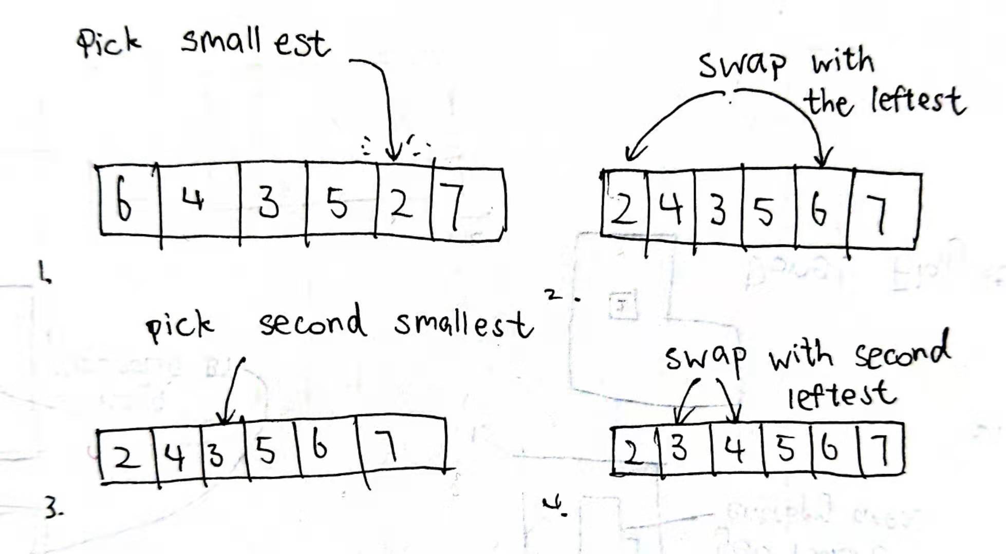
Insertion sort looks a lot like when you play poker, or majhong, or any kind of card games. When you are reassigning your hand, you will pick the smallest card in your hand, and put it to the leftest side; then you will pick the second smallest card, and put it to the second leftest side. And the third, and the forth, … You get what I mean. However, instead of just put it there, insertion sort chooses the old swap. Because in reality, inserting the item over there means all other items should be pushed back by one, and it would mean another iteration, which would really slow down the algorithm. So here’s how it actually works:

However, despite being slightly better than Bubble sort, its performance really didn’t go up that much, and its worst case performance and average performance is still at \(O(n^2)\).

sort it | mix it

And here’s some code, at your disposal:

for (int i = 0; i < array.size(); i++) {
    int minIndex = i;
    int minValue = array[i];
    for (int j = i; j < array.size(); j++) {
        if (array[j] < minValue) {
            minIndex = j;
            minValue = array[j];
        }
    }
    swap(array[i], array[minIndex]);
}

There would be situations when the minimum is just i. If such scenarioes occur, then swap is no longer necessary.

Shell sort

Shell sort is an improved version of insertion sort made famous by Donald Shell. It divides the original array into multiple sections using gaps. It then works down sub-insertion sort from the highest gap to the lowest gap. It’s worst case performance is branched by the choosing of gap, which signifies the importance of gap choosing (duh!): \(O(n^2)\) for the worst known worst case gap sequence, and \(O(n\log^2n)\) for best known worst case gap sequence.

sort it | mix it

So, as we can see here, the first gap is ten: that means the whole array was splitted into ten subarrays, each subarray has two element. We then semi-bubble sort it. Then the gap is five: it was splitted into five subarrays, each with four element. Then two, each with ten elements. Finally, it was devolved into one giant subarray, which has 20 elements, and became our dear Bubble sort.

In fact, Shell sort works just like a gapped Bubble sort: it means for each gap, which in turn means each gapth element, its order will be correct. So at first every 10th element will be in correct order; then every 5th element will be in correct order; then every 2nd element; and finally, every element will be in correct order. As the gap is really big at first, the overall disorder will go down, so the bubble sort at the end will have a better day.

The gap sequence is critical in Shell sort. Shell himself originally uses \([\frac{N}{2^k}]\), but there are lots of variants since then. Hop to the wiki page if you wanna know more.

for (gap : gaps) {
    for (int i = gap; i < array.size(); i++) {
        for (int j = i; j >= gap; j -= gap) {
            if (array[j] < array[j - gap]) {
                break;
            }
        }
        swap(j, j - gap);
    }
}

Quicksort

And here we are for the world famous Quicksort! Everybody learning Data Structure must’ve heard its name (and all sorting algorithms above), it is one of the most efficient sorting methods to this day, widely applied in all sorts of places (Unix, Java, …). It has an average performance of \(O(n\log n)\), and a worse performance of \(O(n^2)\), though that’s pretty hard to come by.

sort it | mix it

Elegant, right? It’s like ballads for… Colored stripes. It’s concept is also really straight forward: divide and conquer. In fact, it should be conquer then divide, but whatever. So here’s the deal:

1. We choose a pivot value
2. We put everything less than the pivot value to the left, everything greater than the pivot value to the right
3. Now the array was splitted into two parts: the less than pivot part, which number ranges from [very low, pivot], and spans from left to pivot; and the more than pivot part, which ranges from [pivot, very high], and spans from pivot to right.
4. For each part, we execute the procedure again. However instead of the whole array, we limit them to their respective index range.

Thus, the array would be splitted by the pivot: the left side is always less than the pivot, and the right side always greater. In those two parts, they will be again splitted by another pivot, the left side is always less than the pivot, and the right side always greater. Which will be again splitted by another pivot, …

Until the array is splitted into those really, really small arrays, and impossible to split anymore. Then the array is sorted! Because the pivot points would always be in correct order, and at the end, nearly every element is a pivot, so yeah, the array would be in correct order.

However, Quicksort has a slight defect: if the array is already in order when the sorting started, that means the pivot point would always be the greatest (at least as is in my demo); which in turn means all elements will be iterated through for nothing, and here its performance will downgrade to \(O(n^2)\). Which is ironic, because it is so good at sorting chaotic arrays.

Quicksort has another downside that it uses stacks. In embedded systems, those might not be the richest available resources. That’s why the quicksort implementation in embedded systems might actually be Shell sort! Isn’t that interesting?

function quicksort(array, lo, hi) {
    if (lo < hi) {
        int p = partition(array, lo, hi);
        quicksort(arary, lo, p - 1);
        quicksort(array, p + 1, hi);
    }
}

function partition(array, lo, hi) {
    int pivot = array[hi];
    int i = lo;
    for (int j = lo; j <= hi; j++) {
        if (array[j] < pivot) { // If lower than the pivot
            swap(array[j], array[i]); // Dump it i
            i++;
        }
    }
    // See, after the loop above, the numbers less than pivot must be in [0, i) now. Which means
    // the numbers greater or equal than the pivot are in [i, hi]. In this way, we partitioned the array.
    // And i is the partition point. Or something like that? I really don't know how to call i. But you know what I mean.
    swap(array[i], array[hi]); // Remember, array[hi] is the pivot
    return i;
}

quicksort(array, 0, array.size() - 1);

Merge sort

Merge sort comes right after Quicksort! They are all divide-and-conquer type, so I guess putting them together is legit. But if I remember correctly, my school didn’t really teach me Merge sort. Well whatever, it isn’t like I still remember any of them anyway, so here we go! Also it isn’t really that hard, as it’s concept is really simple (ripped straight from Wikipedia):

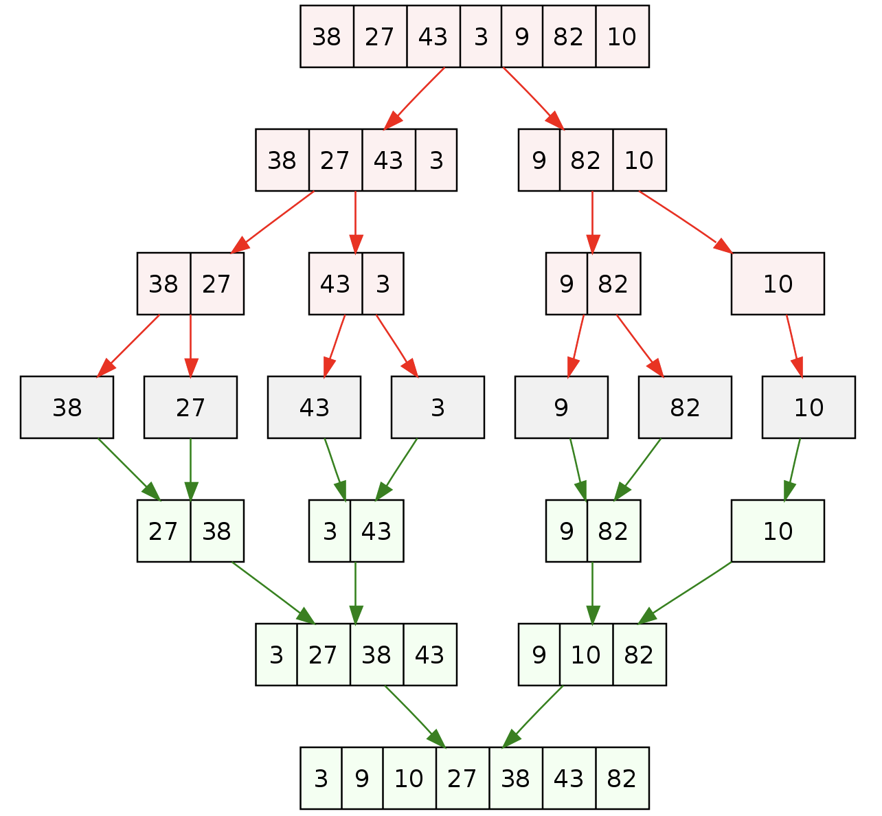
It’s also efficient enough to compete with Quicksort. However, there is no fancy animation for this one: it requires the creation of new arrays, and I am too lazy to write another one. However, as it is fairly easy to understand, it is fairly easy to implement:

function mergesort(array, lo, hi) {
    if (lo + 1 < hi) { // There are at least 2 elements
        int mid = (lo + hi) / 2;
        auto suba = mergesort(array, lo, mid);
        auto subb = mergesort(array, mid, hi);
        return merge(suba, subb);
    } else {
        return array[lo];
    }
}

function merge(suba, subb) {
    int ia = ib = 0; // Index of a & index of b
    auto ret = []; // Please don't care about the terrible pseudocode
    while (ia < suba.size() || ib < subb.size()) {
        if (ia >= suba.size()) { ret.push_back(subb[ib++]); continue; } // If ia is already out of bounds, then the remaining would only be inside subb
        if (ib >= subb.size()) { ret.push_back(suba[ia++]); continue; } // If ib is already out of bounds, then the remaining would only be inside suba
        if (suba[ia] < subb[ib]) {
            ret.push_back(suba[ia++]); // If suba[ia]'s less than subb[ib], suba wins!
        } else {
            ret.push_back(subb[ib++]); // Otherwise subb wins!
        }
    }
}

Merge sort has a worst case, average, and best case performance of \(O(n\log n)\). Even though that makes it seems like it works better than Quicksort, well in some cases, it does; however it does need to allocate new spaces, which is novel in sorting algorithms. Depending on your requirement, you might want that or not.

Heapsort

And here we have another efficient sorting algorithm, Heapsort!

sort it | mix it

Well, the animation would look a little bit weird, because Heapsort itself consists of two different parts:

1. Constructing a “perfect heap”
2. Moving the biggest item (the left one) to the right
3. Reconstruct the “perfect heap”
4. Goto 2

Yeah sorry, that was 4 parts. Well, but 2, 3, and 4 should be counted as one part. So what’s a “perfect heap”? Well, that’s just how I call it really. In Wikipedia, this procedure was called “heapify”, and I guess well, tant pis. Let’s broke it down, anyway:

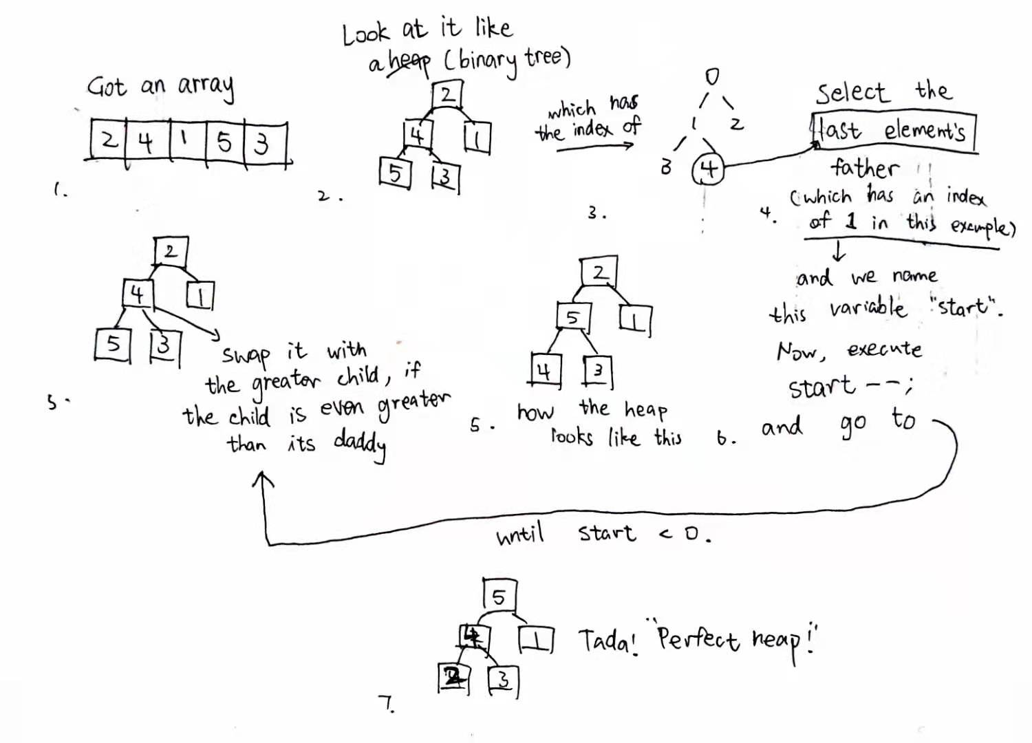
You could notice that this “perfect heap” has an important property which looks a little bit like Quicksort: every node’s child is always less than the node itself. Now that we have this “perfect heap”, everything is nice and easy. It’s like a cone-shaped partial bubble sort over there. Anyway, as we can see in the figure, 5, which is apparently the largest number in my tiny example, is at the top of the tree, which in turn has an index of zero. Now all we need to do is swap the last element with 0!

Now you might notice something uncool. So yeah, we’ve got 5 on the correct order, what now? This heap thing is messed up!

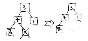
Also notice that as 5 is now in correct order, we really shouldn’t care about it anymore. As a result, we could just think the heap shrinked donw in size, now down to 4. Now, back to what we should do next. You probably know it already. Yep! Reconstruct the great “perfect heap”! This time, four will be on top. Then three. Then two. Then we should stop here, because one will always be correct now. That’s one loop cycle saved!

function heapsort(array) {
    heapify(array); // After "heapify", the array[0] will always be the greatest.

    int end = array.size() - 1;
    while (end > 0) {
        swap(array[0], array[end]); // So we swap it with the last unknown element,
        end--; 
        siftDown(array, 0, end); // And we reconstruct it so array[0] will be greatest again.
    }
}

function heapify(array) {
    int start = father(array.size() - 1); // We start from the tree bottom (or heap top)
    while (start >= 0) {
        siftDown(array, start, array.size()); // By "sifting down", we construct the heap
        start--; // All the way to the top
    }
}

function siftDown(array, int start, int end) {
    int root = start;
    while (leftChild(start) < array.size()) { // While the root still get any child at all
        left = leftChild(root);
        right = rightChild(root);
        int selection = left; // We default the comparison the left child, however
        if (right < array.size()) { // If there is right child, 
            selection = array[left] > array[right] ? left : right; // We will choose the greatest child
        }
        if (array[selection] > array[root]) { // If this child is greater than its father
            swap(array[selection], array[root]); // We swap them
            root = selection; // And we go down a level
        } else {
            return; // Otherwise the heap is for now correct
        }
    }
}

// === HELPERS BELOW === //

function father(int i) { // Father of i
    return (i - 1) / 2; // Notice that precision would be lost, and that's exactly what we want, so regardless of left child / right child, we will get the same result
}

function leftChild(int i) { // Left child of i
    return i * 2 + 1;
}

function rightChild(int i) { // Pretty self explanatory now
    return i * 2 + 2;
}

From the code, we could see that even the heap is messed up, it isn’t that messed up; only the very first row! So we are just going to sift the largest value down below to the top, again moving small values down. There is no need to fully reconstruct the “perfect heap”, just like the first time; we just need to partially reconstruct it.

So, during “siftDown”, we look at one particular node. And if its child are greater than itself, we sink it down to this particular node, and descend into its child (which now has the value of the particular node). In this way, we can make sure that the node’s children are always less than the node itself, as I mentioned above.

Now, take a look back at the animation. At first it’s really just heap constructing. But after the largest value is at the leftest, the actual sorting begins, moving the leftest value to the rightest, and reconstructing the heap every time. Cool!

Heapsort could be complicated. It has a worst case performance and average case performance of \(O(n\log n)\). Well, and that’s it!

Cocktail shaker sort

Well, that’s three efficient sorting methods. Let’s take a break by taking a look at an eye-relaxing (and easy to write) sorting algorithm! That’s Cocktail shaker sort. Now not only does it look good, it actually works better than Bubble sort (even though not soo much)!

shake it | mix it

It’s code didn’t really change much to that of Bubble sort’s, too:

int direction = 1;
for (int i = 0; i < array.size() - 1; i++) {
    while (!(direction == 1 && j >= array.size() - 1) || (direction == -1 && j <= 0)) { // While its comparator would not be out of bounds
        bool shouldSwap = false;
        switch (direction) {
        case 1: // if going right
            shouldSwap = array[j] > array[j + 1];
            break;

        case -1: // if going left
            shouldSwap = array[j] < array[j - 1];
            break;
        }
        if (shouldSwap) {
            swap(array[j], array[j + direction]);
        }
        j += direction; // March to that direction
    }
    direction = -direction; // Reverse direction
}

Alright, there’s a teeny tiny bit of difference. However, it is really not that hard to understand, huh?

Also, I am quite aware that the code here could be optimized. A lot of my code could be optimized, in fact. Well, I am not gonna do it here, but if you know how to optimize, remember to apply that into your code!

Radix sort

After the little hoopla, let’s take a look at this brilliant sorting algorithm that requires no comparison at all: Radix sort! Also called Bucket sort, has a worst case performance of \(O(w\times n)\). Now that’s really low! But of course such brilliant algorithms usually comes with a downside. Well, for one, Radix sort really can’t sort out irrational numbers. A simple example will be enough to walk you through.

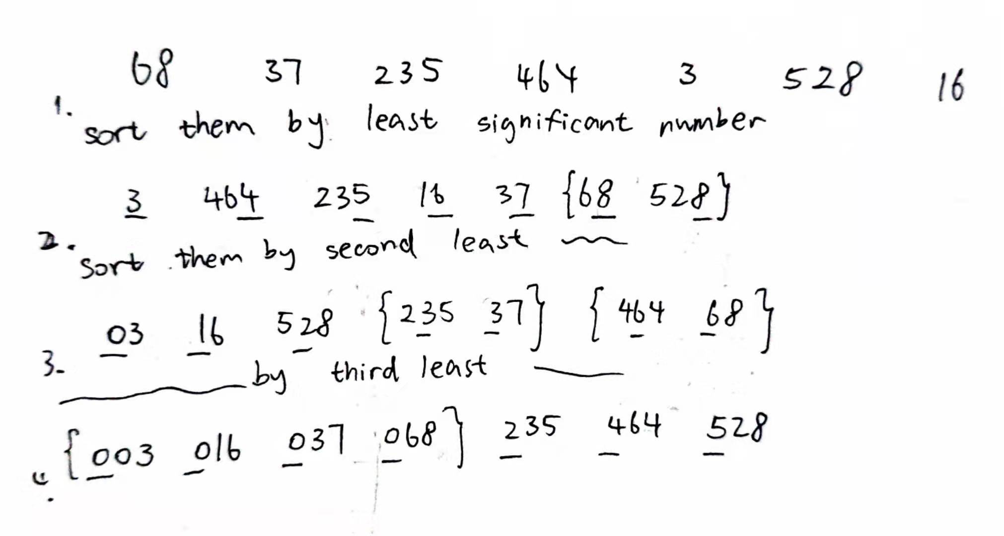
See why Radix sort does not have the ability to sort out irrational numbers now? Because that would require a really really big array, and it didn’t really make sense. Let’s take a look at the procedures!

1. So first we get all these numbers. We iterate through all of them, putting a number to an array with the index of their least significant bit, and we name this array bucket array. So 123 will go to array[3], and 50 will go to array[0], and 127 will go to array[7].
2. Now we iterate through the bucket array’s non-empty indexes, and we look at the second least significant bit. We again put them into another bucket array. 123 goes to array[2], 50 goes to array[5]. 127 also goes to array[2]. Now remember we are iterating through it, so the 123 will go to array[2] first: 127 will follow 123. Now this is how the orderness of raidx sort comes.
3. Finally we iterate through this new bucket array’s non-empty indexes, and we look at the most significant bit (for those three example numbers). 123 goes to array[1], 50 goes to array[0] (0 had been prepended in front of 50: now it’s __0__50). 127 also goes to array[1]. Again, the order does not change.

If you did not find this convincing, take a paper and draw. You will notice how the order forms in Radix array, and how clever its idea is.

bucket = {};
int digits = array.largest().digitCount();
for (int i = 0; i < digits; i++) {
    if (i == 0) {
        for (int j = 0; i < array.size(); j++) {
            bucket[array[i][0]].push_back(array[i]); // The element goes to the corresponding least significant bit sub-array. You know what I mean...
        }
    } else {
        newBucket = {};
        for (bit in bucket) {
            for (int k = 0; k < bucket[bit].size(); k++) {
                int val = bucket[bit][k];
                newBucket[val[digits]].push_back(val);
            }
        }
        bucket = newBucket;
    }
}
// After this procedure, numbers in buckets will be sorted. Just think about a way to iterate them out!

And that’s Radix! Also my implementation might be a little bit wrong, as my memory for this particular implementation is pretty far away. Go look on the Internet!

Bogosort

Alright, and now I am getting tired. Let’s take a look at the sorting algorithm’s ultimate madness: Bogosort!

You must’ve heard of it at some point in your life: The Infinite Monkey Theorem. It means if a monkey could just sit there & type randomly in the typewriter forever, there must be one day when it finally achieves to type out the whole William Shakespeare’s masterpiece. So, if numbers would just switch randomly forever, there must be one day when they will be in correct order, right?

sort it? | mix it

You know, when n is small, its speed is actually pretty quick. And by small I mean 1 or 2? Its worst case performance… Well, let’s say it does not have a worst case performance. It could just go on forever. The average case performance is \(O((n + 1)!)\), and its best case performance, surprise surprise, is \(O(n)\). So power does come at a price, right?

Conclusion

Well, that’s a lot of sorting algorithms! There are more, more sorting algorithm than this, of course; but I am picking a few interesting ones. Also I really am just posting what I know here, and again, don’t assume I am right; assume I am wrong whenever possible. And correct me! Thanks! Also during all those sorting algorithms, I guess we learned that well, Quicksort is called Quicksort for a reason, right?

References

1. Bubble sort | Wikipedia
2. Insertion sort | Wikipedia
3. Shell sort | Wikipedia Actually, all those algorithms are present on Wikipedia.
4. Shell sort in Programiz It has a pretty nice demostration!
5. Quicksort | Wikipedia
6. Quicksort - GeeksforGeeks
7. Merge sort | Wikipedia
8. Heapsort | Wikipedia
9. Cocktail shaker sort | Wikipedia
10. Radix sort | Wikipedia
11. Bogosort | Wikipedia Alright, that’s a lot of Wikipedia entries!
12. the Sorting Algorithm page on Wikipedia Yeah, this is gonna be the last one.
13. Scripts & Stuffs from this post So if you are interested, you can go over there and have a look.

Comments

A valid, non-empty username is required.

Comment