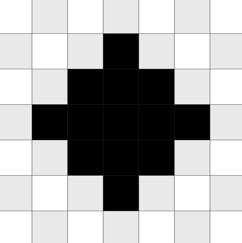
Imagine you have to render a circle in a 6x6 canvas. Given a 2D array representing pixels, you thought up of the solution that the circle can be rendered by evaluating whether each pixel is inside the circle or not.

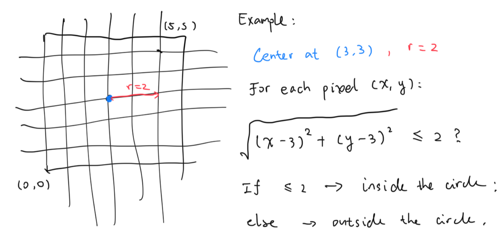
That’s a pretty cool solution, and soon you have your first pixelated circle.

You realized that the determination of whether the sample point is inside the circle is critical in rendering it, and so now you wrap it into a function called inside.

for (int y = 0; y < 5; y++) {
    for (int x = 0; x < 5; x++) {
        if (inside(x, y)) {
            color_black(x, y);
        } else {
            color_white(x, y);
        }
    }
}

You soon realized that by moving the radius to the left side, the function becomes \(\sqrt{(x - 3)^2 + (y - 3)^2} - 2 \leq 0\), which can then be generalized to \(f(x, y) \leq 0\). So long as the \(f\) function is properly defined, every shape can be rendered by executing the generalized code above. For example, a pyramid:

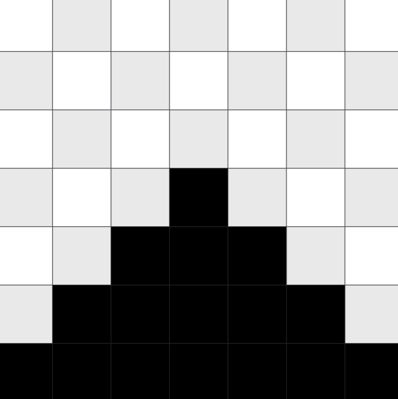
Or a square:

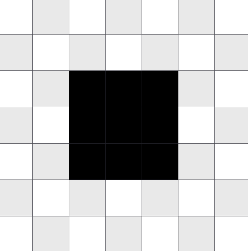
And they are amazing. By searching online for more information, you realized there’s a very similar thing, called implicit functions, which is in the form of \(f(x) = 0\), describing the contour of the shape. So a new question popped up: what if you are to generate the contour of a shape?

Marching Squares

Sure enough, you can just change the inside function into \(f(x) = 0\) and the contour will be rendered, but this becomes tricky when the canvas becomes bigger, and floating point enters the picture. For example, when the canvas space is normalized to [-1, 1), and the implicit function becomes \(\sqrt{x^2+y^2} - \frac{1}{2} = 0\), it’s very, very hard to land onto a pixel and and get exactly 0. This results in severe aliasing and the contour will not be produced at all. Here’s a comparison of the aforementioned circle and the result by changing the inside function comparison from <= to ==:

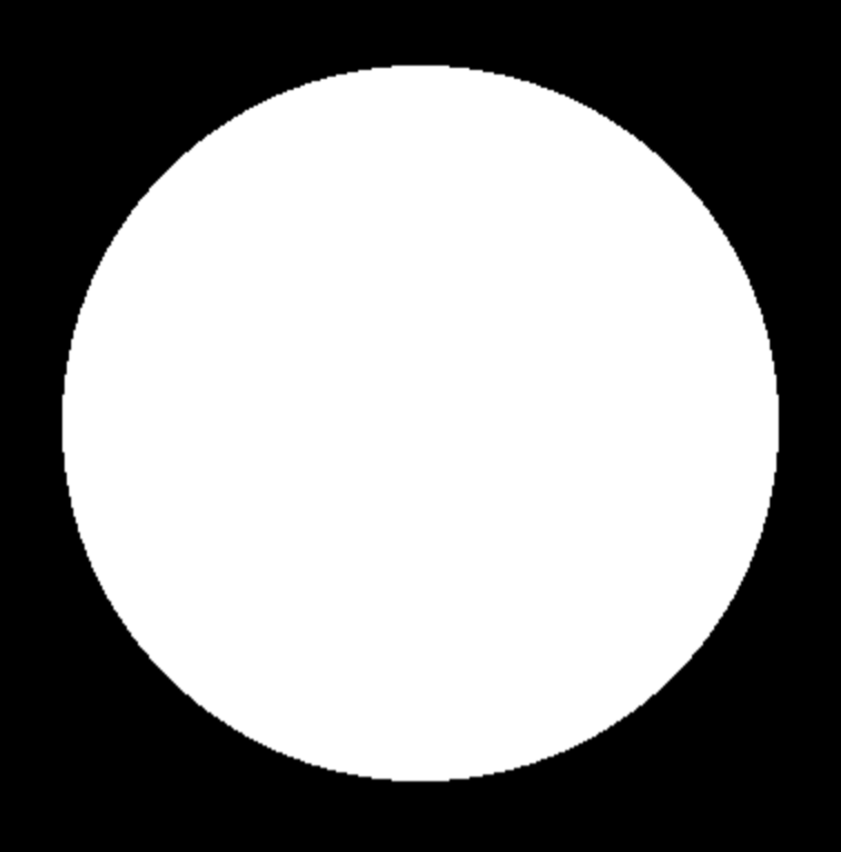
So how do we generate a contour, really? So comes our savior, the marching squares method. And here’s how marching squares work.

First, we divide the canvas into \(w \times h\) cells again. This is called the “resolution” of the marching squares, and we’ll see why is it called like that in a bit.

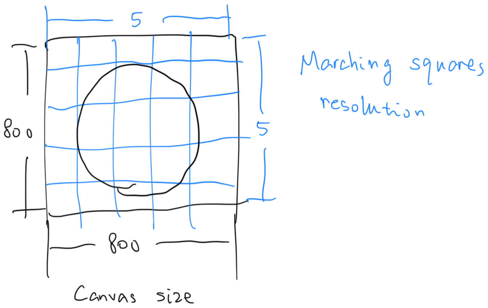
Then, for each cell, we evaluate the inside value for its four vertices making up the cell. Take a look at the example image below.

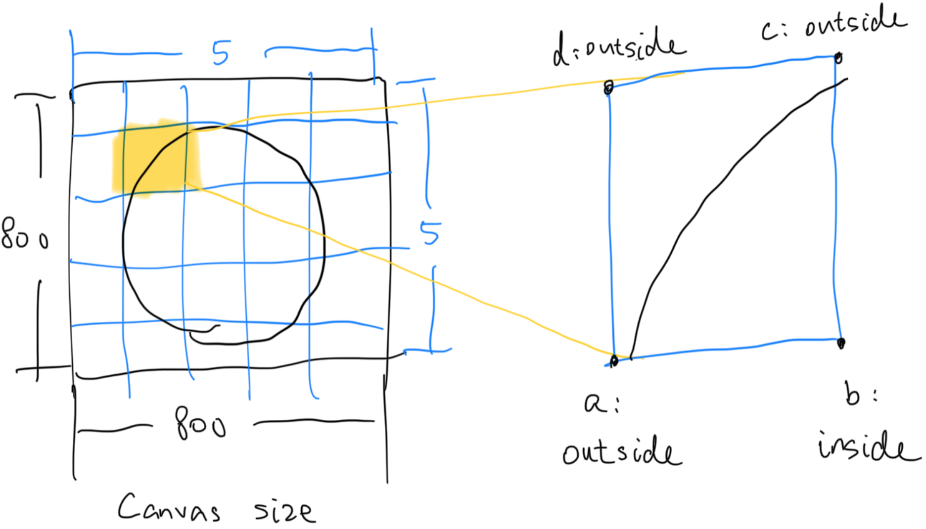
Now let’s enter the local space and disregard our knowledge for the circle. We see that in the cell highlighted above, \(a, c \text{ and } d\) are “outside”, while \(b\) is “inside”. Even if we have no knowledge about the approximate shape of the thing we are trying to contour, we can infer from here that there has to be a curve within this cell, splitting the inside and the outside.

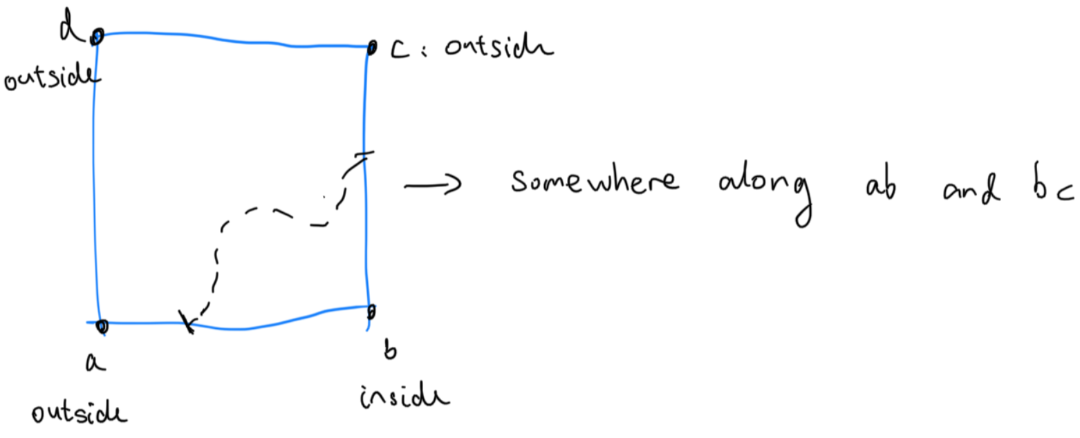
Marching squares just assumes that this “curve” is a straight line, and the two anchor points are right in the middle of \(ab\) and \(bc\). We may be able to infer more information if given more context, but right now since we only have “inside” and “outside” for guidance, that’s the best we could do.

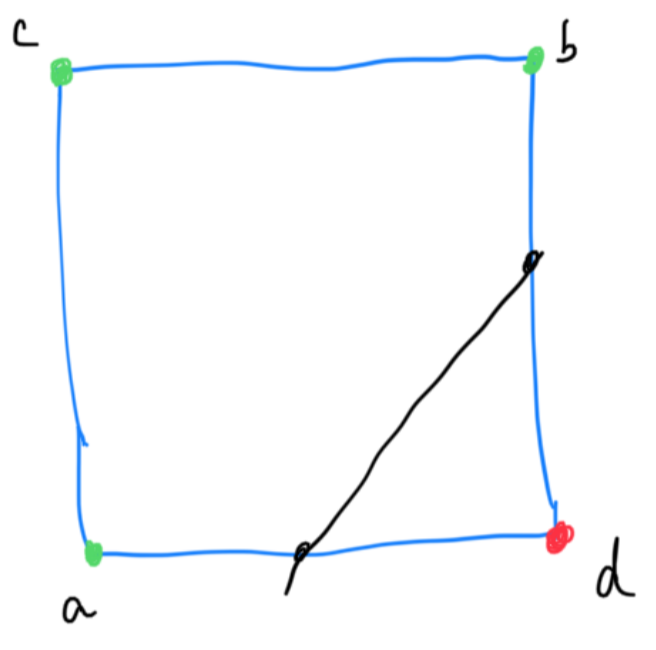
Also from now on, we will use green to denote points that are outside (positive value), and red to denote points that are inside (negative value). If rare occurrences of f(x) == 0 do occur, we treat that as inside as well.

Patterns start to emerge when we consider other possibilities. When both \(a \text{ and } c\) are outside and both \(b \text{ and } d\) are inside, there must be some sort of curve along \(ac\) and \(bd\) dividing the center; and so we draw a straight line through the half point of \(ac\) and \(bd\). When you think about it, with each point only being able to be outside of a shape or inside of a shape, \(a, b, c \text{ and } d\) can only represent so much combinations. Specifically, with 0 being outside and 1 being inside, \(abcd\) can range from 0000 to 1111, and that’s a maximum of \(2^4 = 16\) total possible combinations.

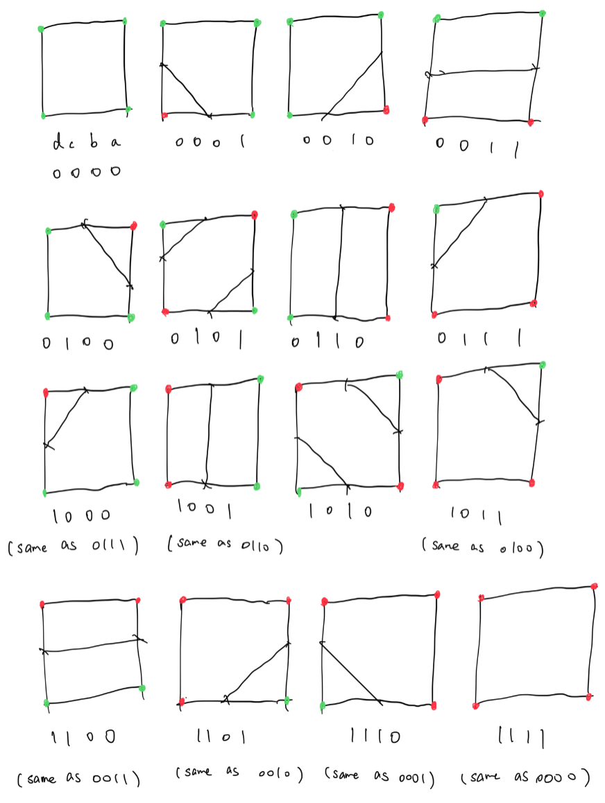
As we can see, when all four vertices are inside or outside, there need not a line separating the cell. Also, when the inside-outside bits are inverted, the pattern is usually the same; the only distinct combination being 1010 and 0101. So in the end, there are 9 distinct patterns.

Wielded with this newfound knowledge, we can now draw the contour of the circle using marching squares.

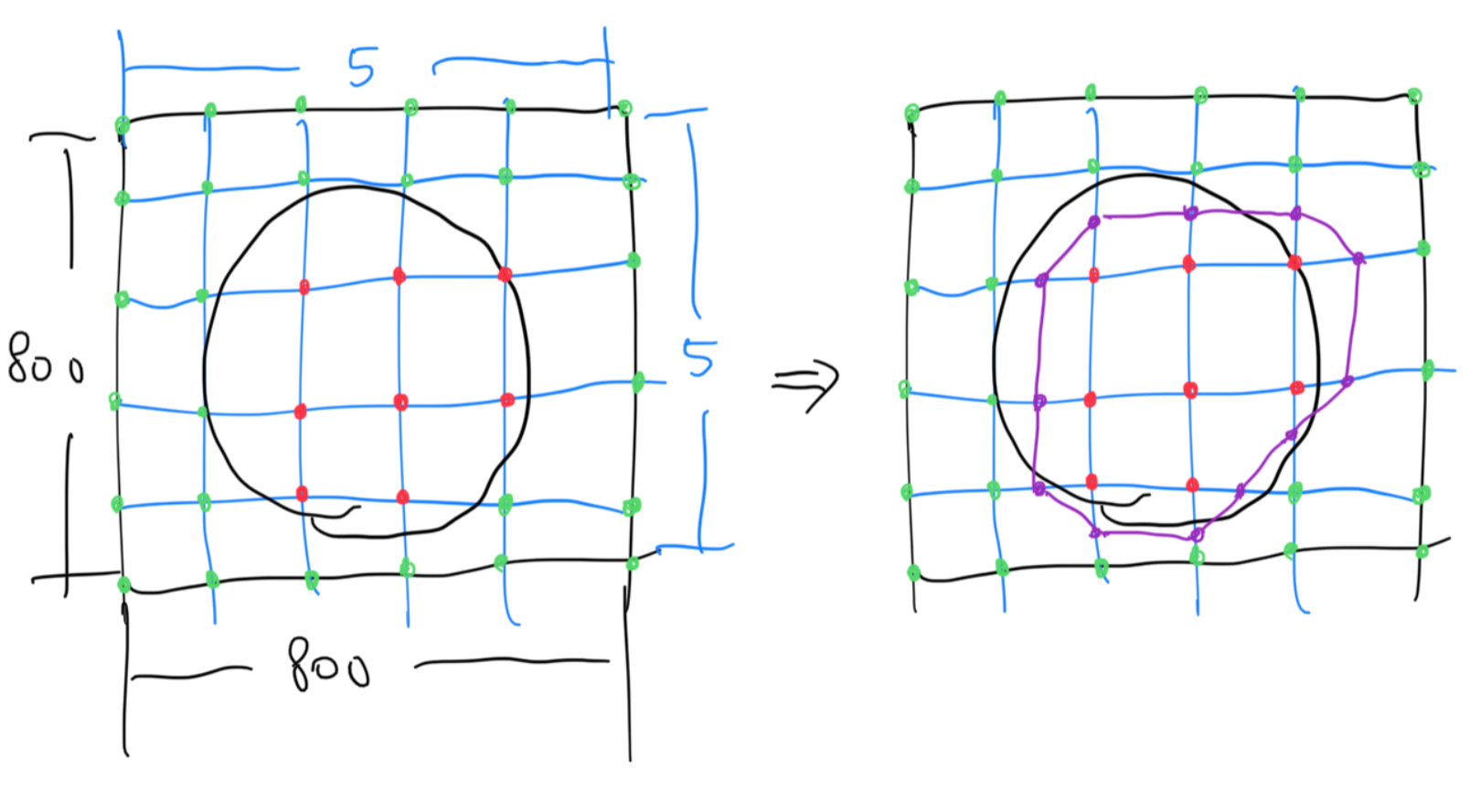
The result is a weird shape thingy. With some contours being completely inside of the circle and some completely outside. However, it is quite easy to imagine that by tuning up the resolution to, for example, 10x10, each cell can achieve higher granularity, and the resulting contour will be better. The marching squares algorithm can be further extended by storing the implicit function value instead of simply storing the inside/outside boolean. We can then interpolate the line vertices between the two cell vertices using the function value instead of just positioning them in the center.

Marching squares is a fine way to transform implicit geometry representation to explicit geometry representation. This can be reflected from the fact that we can store the result vertices, and the next time, we can just draw these lines, dropping the dependency, or the knowledge, of the implicit shape.

Once we get the vertices, we can also perform matrix operations on them: localized rotations and translations are very good properties to have. The marching squares however comes with the inevitable downside of having some information loss. Since the implicit function is continuous, this cannot be avoided. The only two way to lower the aliasing would be increasing resolution, and lowering the function frequency.

Marching Cubes

Now think about marching squares, but in 3D. In the 3D world, we now no longer divide the canvas into little squares, but divide it into little cubes. And now for each cube, there’s 8 vertices instead of 4. It can be inferred that there can be a maximum of \(2^8 = 256\) patterns of something, but surely due to the mirroring rule above, there can’t be this much.

The first question however, is what this something is. In marching squares, the lines are what’s separating the inside from the outside. A simple and intuitive way is to list an example. How about 00000001?

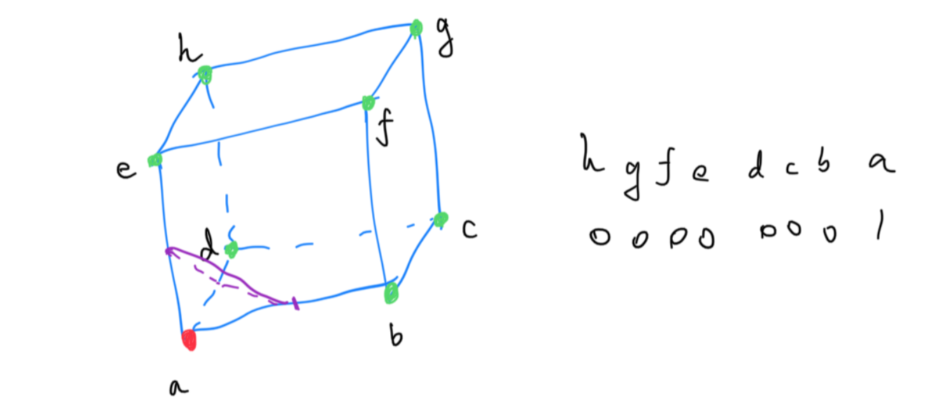
It becomes very obvious from the above image that the divide happens in three dimensions, and therefore, three lines forms a triangle. Which, conveniently, is the base component for 3D mesh and models. That means we can actually export the marching cubes result to Wavefront .obj format and so on. The original paper published by William E. Lorensen and Harvey E. Cline exploited the rotational, reflective symmetry, and sign changes to reduce the 256 combinations into 15 distinct cases. Due to the fact that an explicit representation can also be transformed using matrices, marching cubes becomes very popular in data visualization, especially medical imaging, where layered, implicit, scanned data can be effectively reconstructed into 3D model.

The steps for marching cubes are:

1. Initialize a vertices array for the final mesh.
2. The scene bounding box is divided into \(w \times h \times d\) little cubes, called “resolution”. We divide it based on the scene bounding box so that no wasted calculation is produced.
3. For each cube, we evaluate its eight vertices, and determine whether they are inside or outside.
4. The status of the eight vertices are then used to determine the pattern for this particular cube, and we push the new triangles generated in this cube into the vertices array.

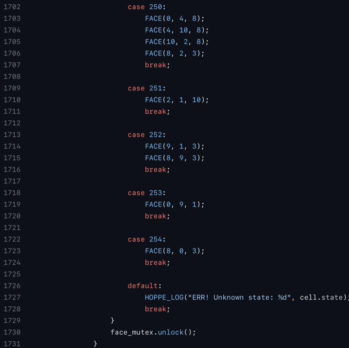
I have written a marching cubes demo here, with all the possible patterns written in a HUGE switch, covering 0-255.

The demo is actually not mesh reconstruction from implicit function; rather, it is mesh reconstruction from point clouds. However, the underlying principles are the same. The method written in my code is an implementation of Hugues Hoppe’s Surface reconstruction from unorganized points, but it is beyond the scope of this post. However, feel free to give it a read if you are interested! This demonstrates marching cubes has way more potential than simply constructing explicit mesh for SDFs (signed distance fields, aka the implicit functions we are referring to above), but also from dense point clouds, and more.

Further Readings

That’s it! Hopefully this post will give you a good intuitive understand of marching squares and marching cubes. If you want to learn more, The Ccoding Train has an awesome video tutorial on how to make marching squares; and Sebastian Lague’s video offers deep insight on marching cubes, and what they can do in video game development: an infinite world generated by a random implicit function.

• Matt’s Webcorner has an explanation on marching cubes as well as the demo source code.
• Paul Bourke’s Polygonsing a Scalar Field has an excellent explanation for marching cubes, which I used as reference when I was writing my marching cubes code.
• The marching cubes on Wikipedia tells the history of how marching cubes come to be, and a brief section on implementation.
• Polycoding also has a blog post on marching cubes, and its implementation in HLSL.

Comments

A valid, non-empty username is required.

Comment