This is a blog post from the past. Originally written at 2020-01-30.
Wave Function Collapse is quite a nice algorithm invented by Maxim Gumin. However, Gumin’s source file could be obscure and hard to understand, so I am writing what I’ve learned so far here, so that I could remember it when it is needed. Also, we are talking about the overlapping model here, not the tiled model (as it is what I am interested in). Sorry! All Wave Function Collapse below refers to Wave Function Collapse, the overlapping model.
Introduction
What is Wave Function Collapse, exactly? This is a concept loosely borrowed from Quantum Machanics. I really advise you to watch this video if you are interested in that kind of stuffs. But here we are talking about WaveFunctionCollapse, the PCG (ProCedural Generation) algorithm. It’s usage is quite simple: You feed it an input image, or whatever looks like an image, and it outputs eerily similar results. Let’s take a look at a few (stolen directly from GitHub repo):
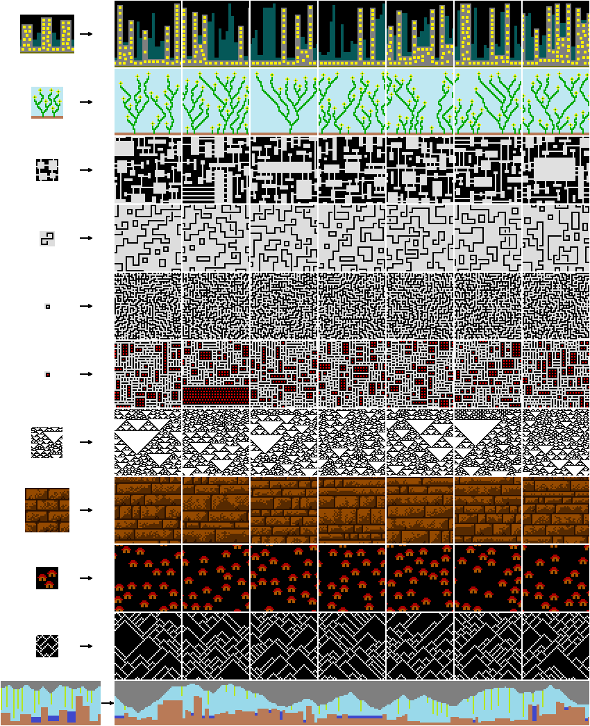
Now, isn’t this cool? Without all sorts of “machine learning” and stuffs, by only solving the constraints, lots of lively stuffs could appear out of nowhere!
Try it out
Now, I’ve implemented one in Javascript. You could play with it for a little bit, however I am not really sure whether my generator could get the same result with Maxim Gumin’s or not. Also I will cap N at 3 (Trust me, you browser won’t want to go beyond). The color stripe at the bottom is the palatte. Use it to switch colors. Beware that if white cells appear, that indicates a contradiction was met, and you need to generate again.
Implementation
Isn’t that cool? The thing I implement almost works, however it has a major drawback: it is extremely slow. Regardless, I think it’s worth spending 3 days? Or how many? Looking into sources and stuffs. So let’s implement it again! I will be using buttload of pseudocodes down below. And hopefully you can understand!
This algorithm, down to its heart, is “constraint solving”, said by Gumin himself. However, 2D map / texture generation is the most mature usage of this algorithm. It could also be used to generate 3D constructions & poetry, as you can see from its project page. But without further ado, let’s look at the core-est procedure:
    int main() {
        getInput();
        processInputsIntoLoadsOfPatterns(N);
        initializeOutput();
        while (notFullyCollapsed()) {
            observe();
            propagate();
        }
    }
That’s it. In a way, it is quite simple. There might be some word you don’t understand there, but don’t worry, we’ll get to it!
Getting input
There are lots of ways to get user input. In C++ you might use “stb_image”, or if you don’t want to use an image (such as if you are a roguelike fan, then why not just cutesy ASCII characters?), you could always implement one yourself. Thus, we are not going to cover this here.
Processing input into loads of patterns
Now here’s an important part. in WFC, patterns are really just a subsection of the original image. This one important parameter, N, stands for pattern size. Such as the thing you drawn above right now (did you)? As its original size is 12x12, if N = 2, there will be at most \([12 - (N - 1)]^2 = 121\) patterns. However, additional patterns will be spawned by rotating around the pattern (which I implemented above), and symmetry patterns (which I did not implement).
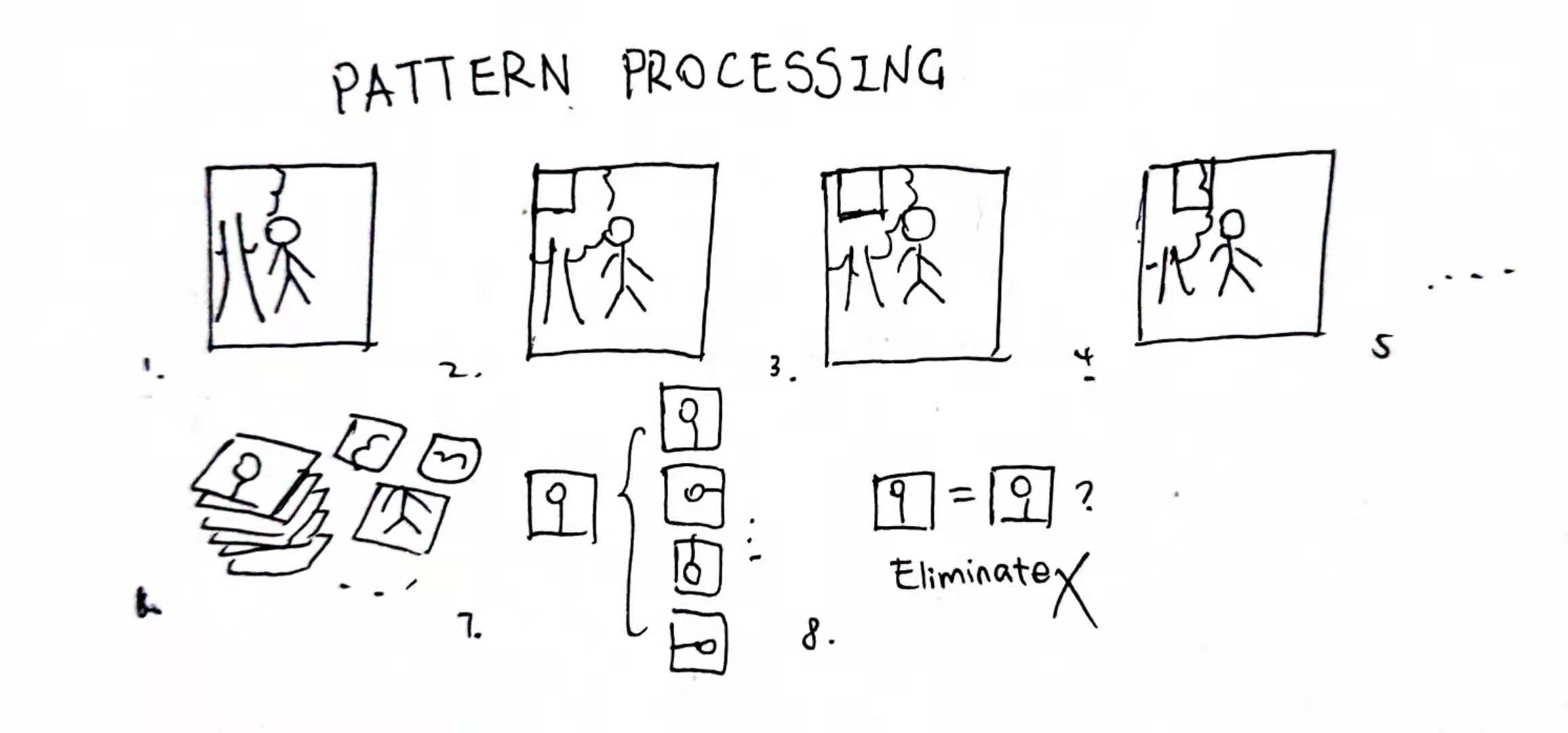
So, the image was chopped up into a lot of (overlapping) little pieces; and then, additional patterns are added by transforming these original little pieces. That would be a LOT of little pieces, and certainly we wouldn’t want that much. That’s why we execute the elimination process at the end; we kill identical patterns, and counting pattern frequency at the same time (as it will be needed later). Using code, it looks a little bit like this:
for (int y = 0; y <= imageHeight - N; y++) {
    for (int x = 0; x <= imageWidth - N; x++) {
        patterns.add(getImageArea(x, y, N, N), "0deg"); // Add the subimage at (x, y), size (N, N)
        patterns.add(getImageArea(x, y, N, N), "90deg");
        patterns.add(getImageArea(x, y, N, N), "180deg");
        patterns.add(getImageArea(x, y, N, N), "270deg");
    }
}
for (int i = 0; i < patterns.size(); i++) {
    for (int j = i + 1; j < patterns.size(); j++) {
        if (patterns[i] == patterns[j]) { // If the pattern is identical
            patterns[i].frequency++; // Count up the frequency
            patterns.remove(patterns[j]); // Delete the identical twin
            j--; // Go back one, so we don't skip the index
            continue;
        }
    }
}
From the code it is not hard to infer that as N goes up, the pattern diversity will increase greatly. And that’s why I don’t want you to go beyond \(N = 3\), that’s enough to lag your browser.
After pattern generation has been done, we need to begin the overlap rule recording phase. That was called propagator in a number of sources, including Gumin himself. However I find that very confusing, so this is what I am gonna call it. Here you should get what I mean, assuming \(N = 2\) (stolen shamelessly from a paper):
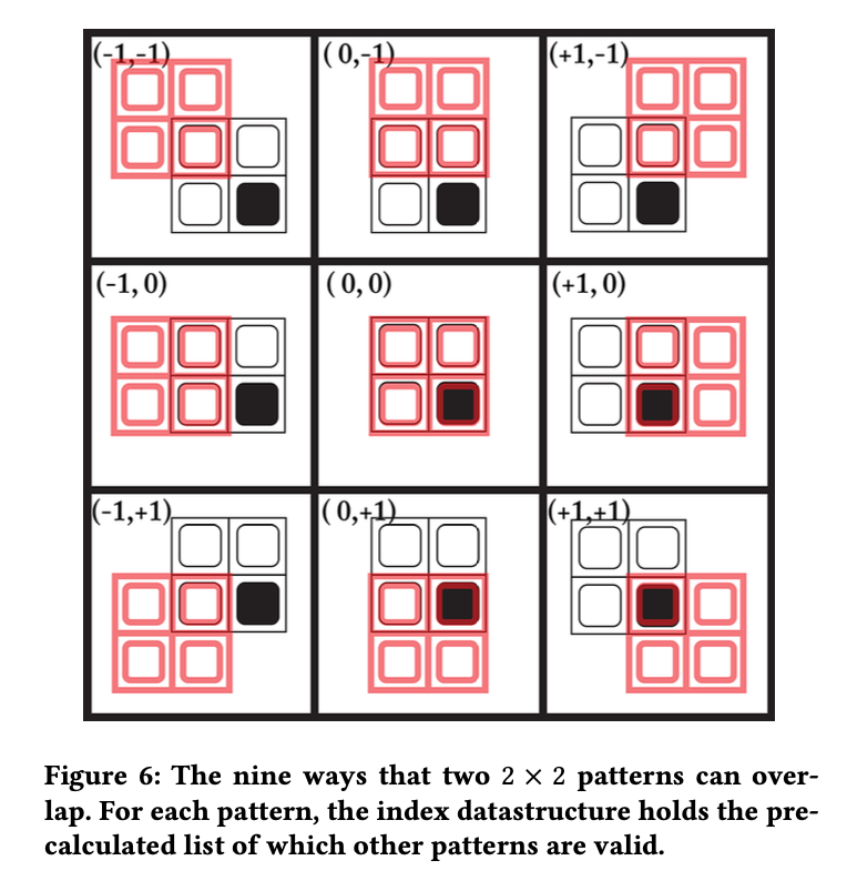
Here as we can see, when N = 2, pattern overlapping could be done in 9 ways. We collect the rules about “when those patterns overlaps, their overlap area is the same” (which is called “agrees” in the original source). So how is that? So here’s another figure, still stolen shamelessly from that paper:
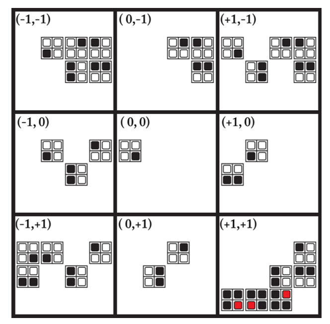
Let’s think about it. When \((dx, dy) = (0, 0)\), the only overlappable pattern with the said pattern is itself. That makes sense, right? Let’s take a look at the figure above, such as when the overlapping pattern is at the original pattern’s (-1, -1) direction: we could see that the only overlapped tile is the original pattern’s top left corner, which is white; and the overlapping pattern’s bottom right corner. Thus, all patterns whose bottom rights are white are allow to overlap with the original pattern, and will be added to the overlapping rules (when offset = (-1, -1)).
After patterns have all been processed, and overlapping rules about each pattern had been added, we move onto the next phase: initialize output!
Initialize output
Be noted that initializing output should only be done after pattern generation is complete. Why? Because in here output isn’t just about initializing an empty image; nope. We are going to initialize a wave! A wave is a two-dimensional array (or any dimension, if you prefer) whose size is exactly the size of the output image’s. Then, for each output cell, we store an array of potential patterns into it (which means all available patterns), in order to mimik it being all those states at once:
for (int y = 0; y <= outputHeight; y++) {
    for (int x = 0; x <= outputWidth; x++) {
        wave.at(x, y) = allPossiblePatterns;
    }
}
Et voila! We got the wave! And we are going to collapse it later.
Entering the loop
As the wave has been initialized, we are about to enter a loop to collapse all those waves, until in each cell, there is only one possible pattern left. If we could reach such circumstance, then a done scenairo happened. What if there is one (or multiple) cells got no possible patterns left? Then we’ve reached a contradiction! But how would we get to those scenarioes? The first thing we do is observe.
Observe
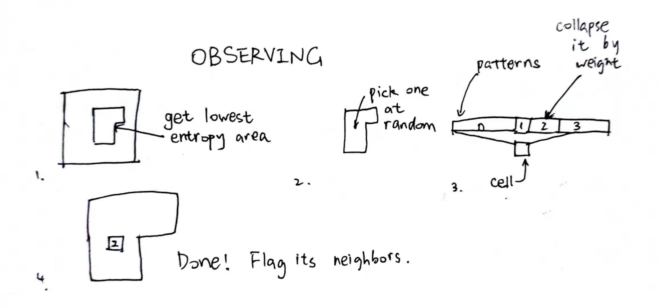
In the double slit experiment, when electrons were not observed, they act as a wave; however when they were observed, they collapsed into a particle (I don’t know if I am saying this correctly, as my profession is not QM). Here we are going to do the same. We observe a random cell, and by doing that I mean collapse a random cell into its definite state. But which cell to collapse?
Well, Gumin is using the “lowest entropy” rule, and so are the others, so we are going to do the same! “entropy” here means the sum of all possible patterns’ frequencies inside a cell. By finding out the lowest entropy cell in the potential output (wave), and collapsing it into a definite state, we could make sure that the effect of this collapse is at minimum (so we don’t have to propagate that much changes).
function findLowestEntropyCells() {
    int currentLowestEntropy = -1; // Undefined entropy at first
    Cell[] cells = []; // Don't care, this is not actual code anyway
    for (int y = 0; y <= outputHeight; y++) {
        for (int x = 0; x <= outputWidth; x++) {
            if (wave.at(x, y).isDefinite()) {
                continue; // We won't want to deal with definite cells; we have observed them already
            }
            if (currentLowestEntropy == -1 ||  // If the lowest is still undefined or
                wave.at(x, y).entropy < currenetLowestEntropy) { // If this one is lower than the current lowest entropy
                cells = []; // we clear the cells
                currentLowestEntropy = wave.at(x, y).entropy;
            }
            if (currentLowestEntropy == wave.at(x, y).entropy) { // This, together with the if above,
                                                                 // means if this cell's entropy is less or equal than the current lowest entropy, we add it to the cells array.
                cells.push(wave.at(x, y));
            }
        }
    }
    return cells;
}
So by executing the findLowestEntropyCells() above, it is quite easy to know the current state of observation. If it returns an empty array, that means we’re done. If it returns an array with minimum entropy of 0, that means we’ve reached a contradictive situation, and the observation has to be put to a stop.
cells = findLowestEntropyCells();
if (cells.size() == 0) {
    return DONE;
} else if (cells[0].entropy == 0) {
    return CONTRADICTION;
} else {
    // We're fine
}
Now, after we found all these lowest entropy cells, it’s time to collapse one of those! Sometimes there will be only one, and we could just collapse it. But what about other times when there are more than one in this array? Well, how about we just let RNG decide! That’s how others do anyway.
cells.chooseOneAtRandom().collapse();
flag(cells.neighbors());
Now, even though choosing which cell to collapse is completely at random, choosing which pattern to collapse to is another story. As we got this “frequency” member in pattern, we could collapse patterns by weight.
Cell::collapse() {
    int e = distribute(0, entropy);
    int i;
    for (i = 0; i < patterns.size(); i++) {
        e -= patterns[i].frequency;
        if (e <= 0) {
            break;
        }
    }
    patterns.splice(0, i); // or patterns.erase(patterns.begin(), patterns.begin() + i)
    patterns.splice(1, this.patterns.length - 1); // or patterns.erase(patterns.begin() + i, patterns.end())
}
Why should we flag its neighbors? That’s because we will need to
Propagate
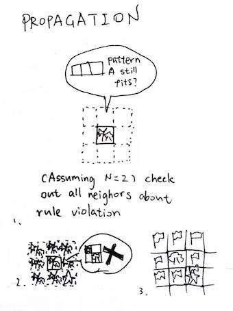
But first, you might wonder: what classifies as a “neighbor”? Well, a neighbor is a potential overlapping cell with the collapsed cell. That would be all cells in [(x - N + 1, y - N + 1), (x + N - 1, y + N - 1)]. Which, in case you didn’t notice, are all the cells in the stolen paper figure 1.
Imagine all flagged cells as an array, so we could get one flagged cell out at a time, like a queue. In fact, the flagged array is a queue. Take one down, propagate around, …
So here’s what we are gonna do: we take a cell down, and iterate through its patterns. Could this pattern be placed here, now that its neighbors are changed? Thus, we check out each pattern’s rules, and if one rule had been violated, this pattern is no longer possible to be placed here, and should be collapsed away.
If this cell’s patterns are also changed, then of course, we should also notify its neighbors. It spreads like wildfire!
while (!flagged.empty()) {
    Cell cell = flagged.pop();
    bool dirty = false; // At first we assume no patterns of this cell has been collapsed
    for (int i = 0; i < cell.patterns.size(); i++) {
        bool legit = true; // At first we assume this pattern of this cell is legit
        for (int j = 0; j < cell.patterns[i].rules.size(); j++) {
            Vec2 offset = cell.patterns[i].rules[j].offset;
            Cell anotherCell = cell.position + offset;
            if (anotherCell.violates(cell.patterns[i].rules[j])) {
                // This pattern could not be placed here anymore.
                legit = false;
                break;
            }
        }
        if (!legit) { // If not legit anymore
            cell.patterns.splice(i, 1);
            dirty = true;
            i--;
        }
    }

    if (dirty) {
        flag(cell.neighbors()); // Yep
    }
}
And by “violating”, it means that no pattern in rules exists in anotherCell.
And that’s the loop!
Let’s review it again:
int main() {
    getInput();
    processInputsIntoLoadsOfPatterns(N);
    initializeOutput();
    while (notFullyCollapsed()) {
        observe();
        propagate();
    }
}
So, unless this whole thing was collapsed (or entered contradiction), we are going to do this forever. Cells will collapse one after another, and each one has a more stricter condition than the last (sometimes). Now there is one question left. As we store patterns into wave, but we need to display pixels, what should we do?
Here’s the place I don’t fully understands… Yet. Gumin uses the following code:
int dy = y < FMY - N + 1 ? 0 : N - 1;
int dx = x < FMX - N + 1 ? 0 : N - 1;
Color c = colors[patterns[observed[x - dx + (y - dy) * FMX]][dx + dy * N]];
bitmapData[x + y * FMX] = unchecked((int)0xff000000 | (c.R << 16) | (c.G << 8) | c.B);
Looks like when x and y is near the border, the color will be the edge of the pattern; otherwise it will be the top left corner of the pattern. I tried it and sometimes its wrong (it must be my problem, yeah), so I am just sampling the top left corner, no matter the position. The great thing is it still works!
If you want to see fancy animations like the one in the GitHub Repo, you could just separate the loop apart, and render it whenever observe() happens. If the corresponding cell has not been fully collapsed yet, you could average its possibilities out, also by sampling all possible patterns’ specific tiles.
Conclusion
So that’s it! Wave Function Collapsed, the overlapping model. I might be wrong, and if I am, please tell me. Also the version I written is, again, extremely slow. So don’t use mine! Use the others! I am using the others as well. And there you have it!
References
- Awesome paper that I stole: WFC Is Constraint Solving In The Wild: It is really awesome!
- GitHub Repository
- Procedural Generation with Wave Function Collapse
- The Wavefunction Collapse Algorithm explained very clearly
- The Very Simple Tiled Model by Robert Heaton
- EasyWFC, an C# implementation
- FastWFC, an C++ implementation (I still don’t know how could it be this quick)
- My bad C++ implemention, for ASCII chars And by bad I mean really bad. Generating a 100x100 map takes 2 minutes.
- My JavaScript implementation Well… It is kinda embedded into the blog source tree. It is also pretty bad, by the way.
Comments