Normal maps contain crucial information about the scene & geometry. It is, as a result, very important in photogrammetry and 3D reconstruction, where we need to recover shape from an image. Sure, there are a lot of other methods, such as the Structure from Motion (SfM) pipeline, with sophisticated tools like OpenMVG, OpenMVS, et cetera, and nowadays there are cooler methods that uses neural networks (who doesn’t love neural networks?) But today, we are going to see how cool & strong normal maps really are by getting our hands dirty and recovering shape directly from a integrating normap map, and discuss this method’s heavy limitations and constraints.

This is gonna be a math-heavy blog, but none of them are too hard. So buckle in!

Depth Maps

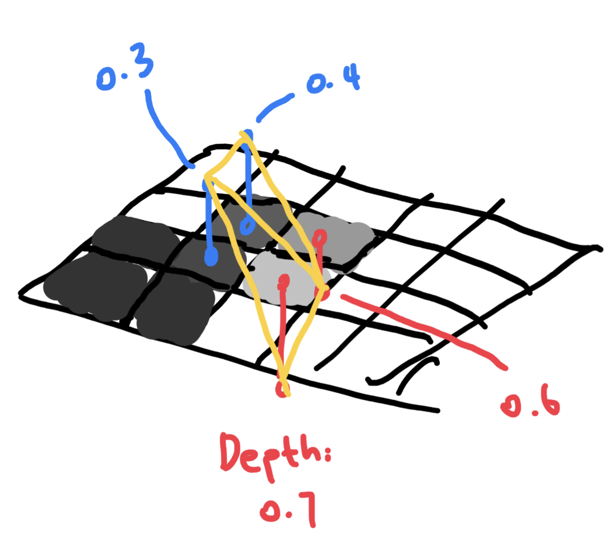
Depth maps contain basically scene information. Why? Because we can just take a depth map, and for every point \(\begin{bmatrix}u \\ v\end{bmatrix}\), sample for

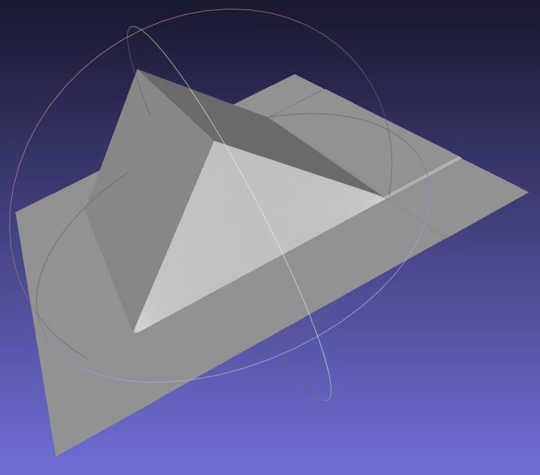
\[p = \begin{bmatrix}u \\ v \\ z(u, v)\end{bmatrix}\]

for its four neighbors. We can then just connect them into triangles and BOOM! We have recovered the scene. Like this:

Since we can reconstruct mesh using a depth map, now our problem becomes: how can we recover depth map from normal map?

Orthographic Camera

Think about an orthographic camera. For every point in a depth map, we can re-project from image plane to the world like this:

\[p(u, v) = \begin{bmatrix}u \\ v \\ z(u, v)\end{bmatrix}\]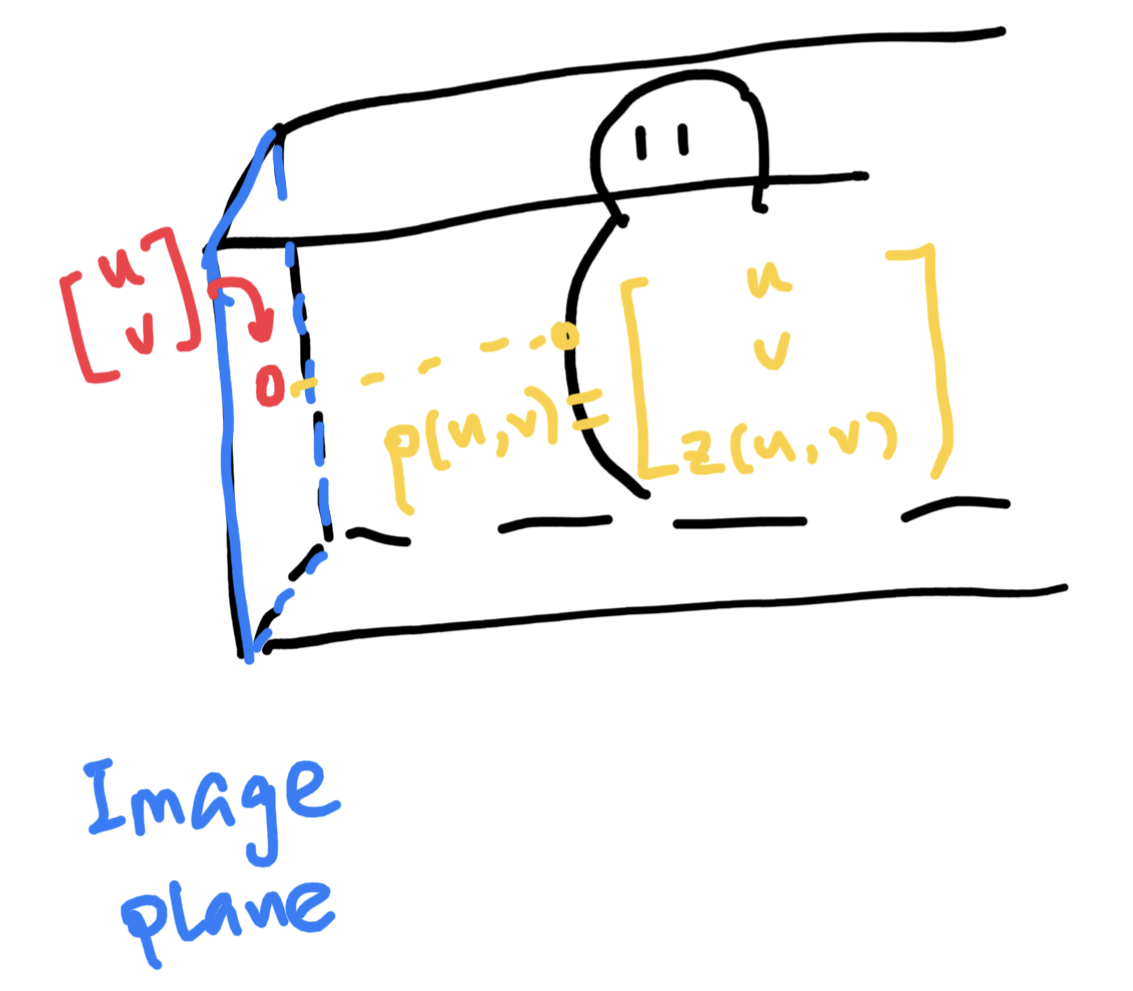

Assuming the principle point is located at \(\begin{bmatrix}0 \\ 0\end{bmatrix}\). For every point p, a normal n is defined. Assuming we have a normal map, normal n for point p would be

\[n(u, v) = \begin{bmatrix}n_1(u, v) \\ n_2(u, v) \\ n_3(u, v)\end{bmatrix}\]

where \(n_1, n_2, n_3\) are just the three color channels of the normal map. To make writing easier, we are going to drop the u and the vs. Now, if we take the partial derivative of p along u and v, we get two vectors that are perpendicular to the normal vector n:

\[\begin{cases} \langle \partial_u p , n \rangle = 0 \\ \langle \partial_v p , n \rangle = 0 \\ \end{cases}\]

The partial derivative of p along u and v are

\[\begin{cases} \partial_u p = \begin{bmatrix}1 \\ 0 \\ \partial_u z\end{bmatrix} \\ \partial_v p = \begin{bmatrix}0 \\ 1 \\ \partial_v z\end{bmatrix} \\ \end{cases}\]

respectively. Plugging them into the dot operations above yields

\[\begin{cases} n_1 + n_3 \partial_u z = 0 \\ n_2 + n_3 \partial_v z = 0 \end{cases} \rightarrow \begin{cases} \partial_u z = -\frac{n_1}{n_3} \\ \partial_v z = -\frac{n_2}{n_3} \end{cases}\]

And now, given an initial depth value \(z_0 = \begin{bmatrix}0.5 \\ 0.5\end{bmatrix}\), we can reconstruct the whole depth map by using

\[\begin{align} z(u, v) &= z_0 + \int_{r}^u \partial_u z dr + \int_{s}^v \partial_v z ds \\ &= z_0 + -\int_{r}^u \frac{n_1(r, v)}{n_3(r, v)} dr -\int_{s}^v \frac{n_1(u, s)}{n_3(u, s)} ds \end{align}\]

…and there we have it! we have successfully recovered depth map from normal map. Triangulating it is simple enough; mesh comes soon after.

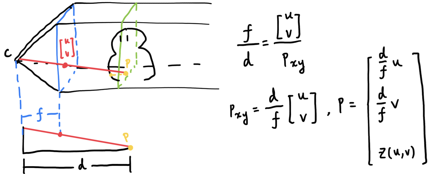
Weak-perspective Camera

We have only covered about the orthographic case so far, and the mesh we’ve recovered is very satisfactory. So let’s move on to the weak-perspective camera. A weak perspective camera is not a real perspective camera, it’s more like when you are looking at the sun, which although is a perspective view, it’s way too far for that to matter, and as a result, acts more like a orthographic camera.

In a weak-perspective camera, the points are first projected onto a plane, located d units away from the focal point; then it is scaled to make far away things small.

It is as a result, trivial to update the PDEs we obtained above:

\[\begin{cases} \frac{d}{f} n_1 + \partial_u z n_3 = 0 \\ \frac{d}{f} n_2 + \partial_v z n_3 = 0 \end{cases} \rightarrow \begin{cases} \partial_u z = - \frac{d}{f} \frac{n_1}{n_3} \\ \partial_v z = - \frac{d}{f} \frac{n_2}{n_3} \end{cases}\]

So, not much different than our orthographic camera.

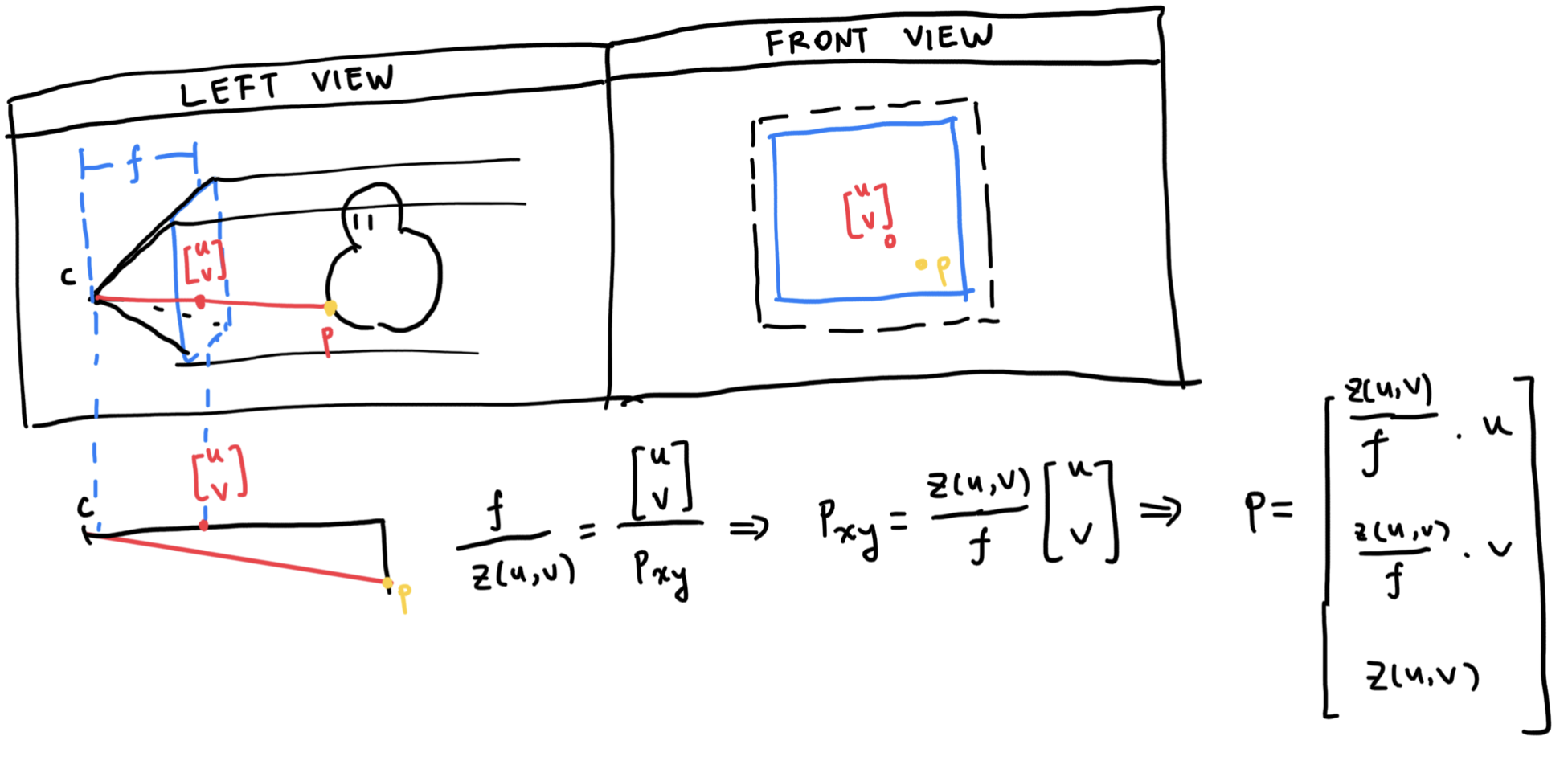
Perspective Camera

Here’s where the fun begins. The perspective camera requires a lot of mathematic heavylifting, due to the perspective nature requiring depth to be part of the equation.

In order to obtain similar PDEs like above, we introduce the concept of a log depth map \(\tilde{z} = ln(z)\):

\[\begin{align} z &= e^{\tilde{z}} \\ \partial_u z &= e^{\tilde{z}} \partial_u \tilde{z} \\ &= z \partial_u \tilde{z} \end{align}\]

With this property in hand, we plug it into the p’s partial derivative above, which yields

\[\partial_u p = \begin{bmatrix} \frac{z}{f} (\partial_u \tilde{z} u + 1) \\ \frac{z}{f} v \partial_u \tilde{z} \\ z \partial_u \tilde{z} \end{bmatrix}, \partial_v p = \begin{bmatrix} \frac{z}{f} u \partial_v \tilde{z} \\ \frac{z}{f} (\partial_v \tilde{z} v + 1) \\ z \partial_v \tilde{z} \end{bmatrix}\]

Putting those back into the dot equation and we get

\[\begin{cases} z (n_1 \frac{1}{f} (\partial_u \tilde{z} + 1) + n_2 \frac{1}{f} v \partial_u \tilde{z} + n_3 \partial_u \tilde{z}) = 0 \\ z (n_1 \frac{1}{f} u \partial_v \tilde{z} + n_2 \frac{1}{f} (\partial_v \tilde{z} + 1) + n_3 \partial_v \tilde{z}) = 0 \end{cases}\]

Assuming z cannot be equal to zero, it cancels out, and we can further simplify this and get

\[\begin{cases} \partial_u \tilde{z} (u n_1 + v n_2 + f n_3) = - n_1 \\ \partial_v \tilde{z} (u n_1 + v n_2 + f n_3) = - n_2 \\ \end{cases}\]

Moving everything to the right except the partial derivative variables and we can get the final result

\[\begin{cases} \partial_u \tilde{z} = - \frac{n_1}{u n_1 + v n_2 + f n_3} \\ \partial_v \tilde{z} = - \frac{n_2}{u n_1 + v n_2 + f n_3} \\ \end{cases}\]

Denoting \(u n_1 + v n_2 + f n_3\) as \(\tilde{n_3}\) and we have successfully unified all equations:

\[\begin{cases} \partial_u \tilde{z} = - \frac{n_1}{\tilde{n_3}} \\ \partial_v \tilde{z} = - \frac{n_2}{\tilde{n_3}} \\ \end{cases}\]

We can now recover perspective and orthographic camera normal maps. The only difference being after recovering a perspective depth map, we need to exponentiate it to get the real depth map.

Results

Let’s take a look at the results! I have only implemented orthographic camera case, but according to the formula presented above, it’s not too hard to extend the code to perspective and weak-perspective cameras.

First, a slope: we can see the slope has been recovered pretty well.

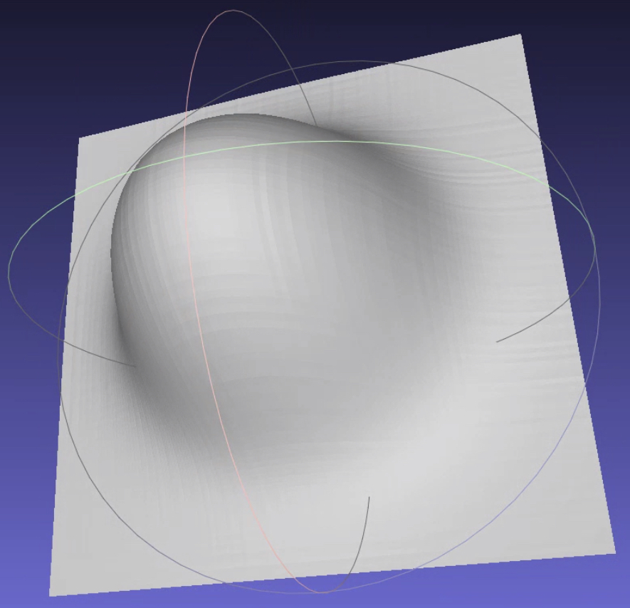
Then, a small mound. This is done by combining a sphere and a plane using the smin function provided by Inigo Quilez:

I have written the code to recover mesh from normal maps, from start to finish. You can check out my code here.

Problems and Constraints

You might’ve noticed the normal maps above are pretty trivial, and you would be right. The method above, the real normal integration method, cannot recover depth map of complex scenes; the reason is due to occlusion, and normal discontinuities, the integration can almost never obtain correct results, or, the depth might change violently when the z component of the normal vector is small; a division-by-zero error might even occur when \(n_3 = 0\).

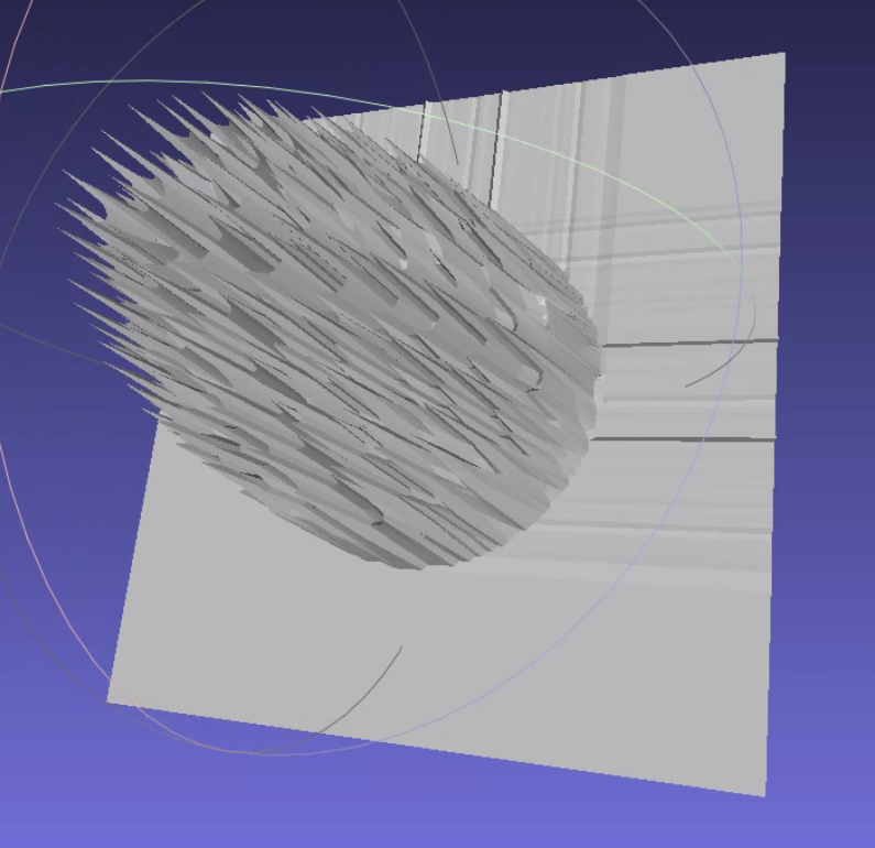
By changing the smooth mound to a hard min of sphere and plane, the mesh recovered now looks terrible:

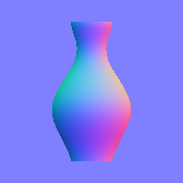
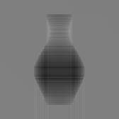
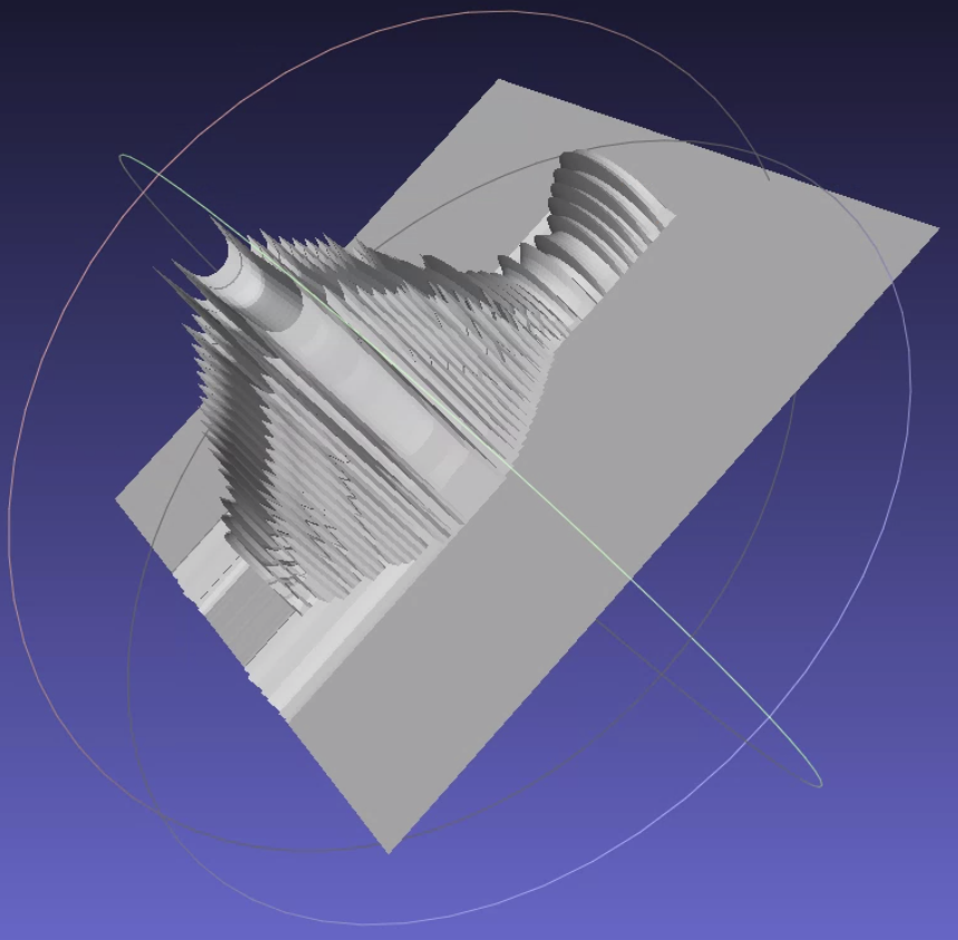
Or take a look at this vase. Also due to the hard min, the end result is less than ideal:

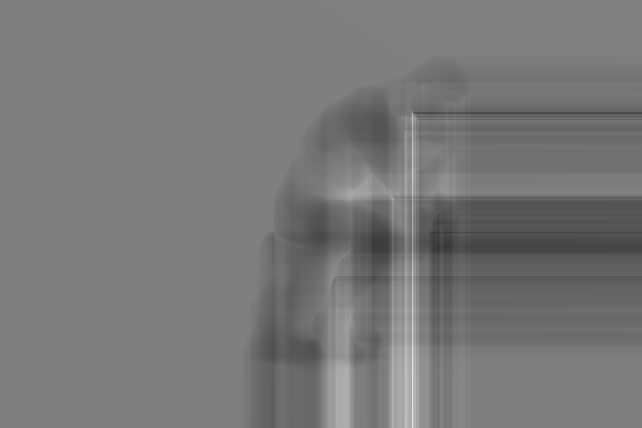
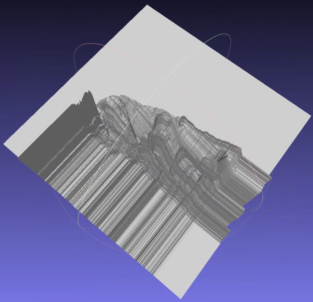
Or, and let’s take a step further, take a look at this thinker normal map presented in the Bilateral Normal Integration (BiNI) paper. As we can see, there is no thinker in the mesh.

Optimization

So yeah, only in very ideal situations, such as those specific normal maps I presented above, where the normal map is continuous, no occlusion is presented in the scene, no extreme normals with a small z value, etc., can the algorithm work well.

But is the normal integration method beyond hope? Of course not! Even though we cannot recover (most of the) depth maps, we can utilize the PDEs and change it into a functional. By minimizing the functional, we can obtain the original depth map itself:

\[\mathcal{F}_{\text{L2}}(z) = \int\int ||\nabla z(u, v) - g(u, v)||^2 dudv\]

The quadratic functional can also be written as

\[\underset{z}{\min} \int \int (n_3 \partial_u z + n_1)^2 + (n_3 \partial_v z + n_2)^2 dudv\]

Most of the normal integration methods nowadays uses this method, but those are already beyond the scope of today’s post. If you want to know more, please check out the reference section, which is like one line away.

References

• Normal Integration: A Survey: introduces the normal integration this post presents, and a few other methods using optimization
• Normal Integration via Inverse Plane Fitting: presents a normal integration method that solves an inverse problem of plane fitting.
• Bilateral Normal Integration (BiNI): studies the discontinuity preservation problem of normal integration and provides a solution; instead of continuous, this paper assumes the normal map is one-sided continuous.
• Simplified Camera Projection Models: introduces a few camera projection models.