ReSTIR is an importance sampling method, which is so powerful you can render the whole scene realisitcally with just 1 sample per pixel (1spp). The original paper is available here. Before we begin, let’s take a look at its impressive result.

There are a few pieces of prerequisite knowledge, but worry not! We will go over it bit by bit. So let’s go!

Monte Carlo Estimator

To solve the Rendering Equation, we can (and have to) use the Monte Carlo estimator. It turns any form of integration from

into

However, we can’t really just use that; poor, uniform sampled random variable \(x_i\) means a poor integration result. Especially when we need to solve the equation in real time , requiring high computational power, we want those samples to count.

Importance Sampling

Let’s take a look at importance sampling. It’s just a slight variation of the Monte Carlo estimator, allowing us to generate samples from non-uniform PDFs, while maintaining an unbiased result:

Now we can generate samples from a PDF that (probably) aligns better with the Rendering Equation distribution. The better they are aligned, the less samples we need to take to achieve an accurate estimate, with the extreme case being one sample. Let’s take a look at why.

If we want to integrate, say, \(\int_0^\pi sin(x) dx\). We pick a PDF that is a normalized version of the function, \(p(x) = \frac{sin(x)}{2}\). Now we generate a sample from this using inversion sampling, which looks like this:

So now some random sample has been generated, say, \(\frac{\pi}{2}\). Plugging it into our importance sampling estimator, we get

Wow. So, the better the PDF aligns with target distribution, the better the integration result with fewer samples. And why is that? Because explained in simple terms, to normalize the distribution, we have to divide the whole function with its integration result.

Multiple Importance Sampling (MIS)

Multiple Importance Sampling is a sampling technique from Veach’s thesis. I haven’t read it myself, but I heard it’s really good.

Imagine we are rendering a scene. Now, although importance-sampling the from light direction or the BRDF can both result in a better integration result, it’s not always the best; if we are shading a diffuse surface and there are two light sources, one big and one small, neither directly sampling from the light direction nor sampling from the BRDF can result in the best performance & accuracy. Ideally the best result would be sampling their combined PDF, but it’s just infeasible to get the PDF for both light direction & BRDF (since getting the precise PDF requires integrating the Rendering Equation, which is a chicken & egg problem.) What should we do?

Introducing the Multiple Importance Sampling (MIS), which tries to tackle this problem:

1. Take M PDFs
2. Draw N sample points from each PDF
3. Perform mini Monte-Carlo integration for each PDF, except:
4. Weight each sample contribution by multiplying it with \(w_i(x_{ij})\)

For each mini Monte-Carlo integration, the weight needs to satisfy

Translating that back into human language, that means

1. The weighting functions among different PDFs should sum to one given a sample point;
2. Weighting function for PDF i at point x should be 0 if the PDF i at point x is zero; this is used to prevent division by zero error.

Suppose we have three different PDFs and we one sample from each (\(x_{11}, x_{21}, \text{and } x_{31}\).) The estimator now looks like this:

If the weighting functions are constant over the whole domain, this becomes

Where \(w_1 + w_2 + w_3 = 1\). But this performs poorly when any of the given PDF is bad, because variance is additive, and any bad PDF among \(p_1, p_2, \text{and } p_3\) will result in a poor estimation.

And so, as a result, choosing a weight function is apparently very important. One of those is balance heuristic:

Plugging it back into the MIS equation yields

Looking back at our previous example, if we use balance heuristic, it becomes

If the first PDF aligns pretty well with f near the region of x, then the \(f(x)\) result will be big as well as \(p_1(x)\); as a result we will count towards its contribution more in this scenario.

Sampling Importance Resampling (SIR)

Sampling Importance Sampling (or Sequential Importance Resampling, also SIR) is a sampling technique that works like this:

1. I have a target PDF \(\hat{p}(x)\) that is hard to draw samples from. (Inversion sampling is expensive sometimes.)
2. I have a proposal PDF \(p(x)\), which looks a little bit like the target PDF, and drawing samples from that is cheap
3. Draw M samples from the proposal PDF
4. For each sample taken, assign weight to it: \(w(x_i) = \frac{\hat{p}(x_i)}{p(x_i)}\)
5. Draw one (1) sample from the sample pool. Probability of a sample being drawn is proportional to its weight.

A few strong benefits can come from using SIR:

1. We don’t need to know how the target PDF looks like, we just need to know how to evaluate it
2. Add a constant scaling factor on target PDF and the result will remain the same

Point 2 is very useful since the target PDF doesn’t even need to be a PDF now. It might as well be any distribution, which, coincidentally, the Rendering Equation without the integration is a distirbution as well!

Remember the one-sample talk we had earlier? Now we don’t need to integrate the function in advance, because PDF is retrieved from normalizing the distribution, which means dividing the distribution by its integrated result over the whole domain. With SIR, we can now generate samples from all kinds of weird, unknown PDFs.

However, SIR is not the holy grail and its downsides are also pretty obvious:

1. Not trackable, as in no closed-form SIR PDF.
2. The first downside leads to the second; non-trackable PDF means we can’t use things like balance heuristic, since that requires evaluating the PDF of SIR
3. Sometimes we need a lot of proposal samples to achieve a good approximation. And sometimes, proposal samples are not that cheap as well.

Resampled Importance Sampling (RIS)

Resampled Importance Sampling, proposed by Justin Talbot, opens up the possibility of exploting SIR to evaluate the integration result of the target PDF. Here’s how it works:

1. Draw M samples from the proposal PDF \(p(x)\) with weights attached
2. Draw N samples with replacement (so there can be duplicate samples) from the sample pool M
3. Sum them up with a bias correction factor. The formula is given below.

The weights in bias correction factor for each sample point in SIR sample pool is

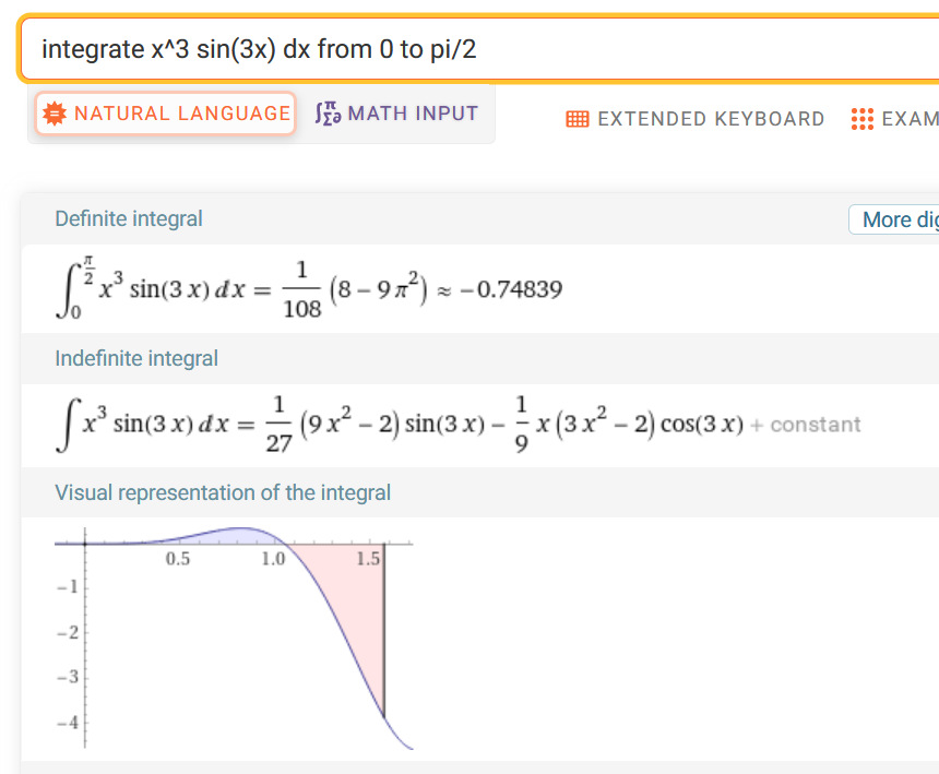
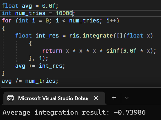
Let’s take a look at an example. Suppose we have a integrand that is basically impossible to know, say, \(f(x) = x^3 \sin(3x)\), and we want to integrate it from 0 to \(\frac{\pi}{2}\). Here’s what Wolfram Alpha says:

In practice, we don’t know what’s inside f(x), but we do have a vague idea of how it might look like, since it should at least kind of resemble \(\hat{p}(x) = x^3\). This can be our target distribution. Although in our example, \(x^3\) is pretty easy to sample from, in reality, the target distribution sampling procedure can also be nontrivial: maybe it’s the combined light incoming directions, or something else. That’s when the proposal PDFs come in, which is quick and easy to sample, such as 1 direct light. Or in our case, \(p(x) = \sin(x)\).

Picking \(\sin(x)\) here is just for demostration purposes; I use the sine PDF to show that any PDF can be picked while using RIS. It’s just bad proposal PDF means more samples.

Anyway, here’s what we have so far:

1. A function to integrate \(f(x) = x^3 \sin(3x)\)
2. A target distribution, \(\hat{p}(x) = x^3\)
3. A proposal PDF, \(p(x) = \sin(x)\)

Note that \(\int_0^{\frac{\pi}{2}} \hat{p}(x)\) doesn’t even equal to one. And here’s when RIS shows its magic:

1. M SIR samples are taken using the inversion sampling method according to \(p(x)\), and each of them have a weight attached to them \(w(x_j) = \frac{\hat{p}(x_j)}{p(x_j) M}\)
2. N RIS samples are taken from the SIR samples proportional to its weight
3. Estimate the integration result \(\hat{I} = \frac{1}{N} \sum_{i=1}^N \frac{f(x_i)}{\hat{p}(x_i)} \sum_{j=1}^M w(x_j)\)

In our case, let’s set \(N = 1\) so we evaluate the RIS integration from a single sample. The result? Even though most of the time it got the answer wrong, we only ever need 1 sample (for RIS), and the integration is unbiased, and converges to our desired result:

In reality RIS is really just a special form of importance sampling, and as a result, can be used by MIS as part of its sampling strategies:

Where \(w^{\text{RIS}}\) is the bias correction factor \(\sum_{j=1}^M w(x_j)\). Note that the M here means different things, in the MIS formula above the M means number of sampling strategies, and in the \(w^{\text{RIS}}\) it means number of samples drawn from the proposal PDF.

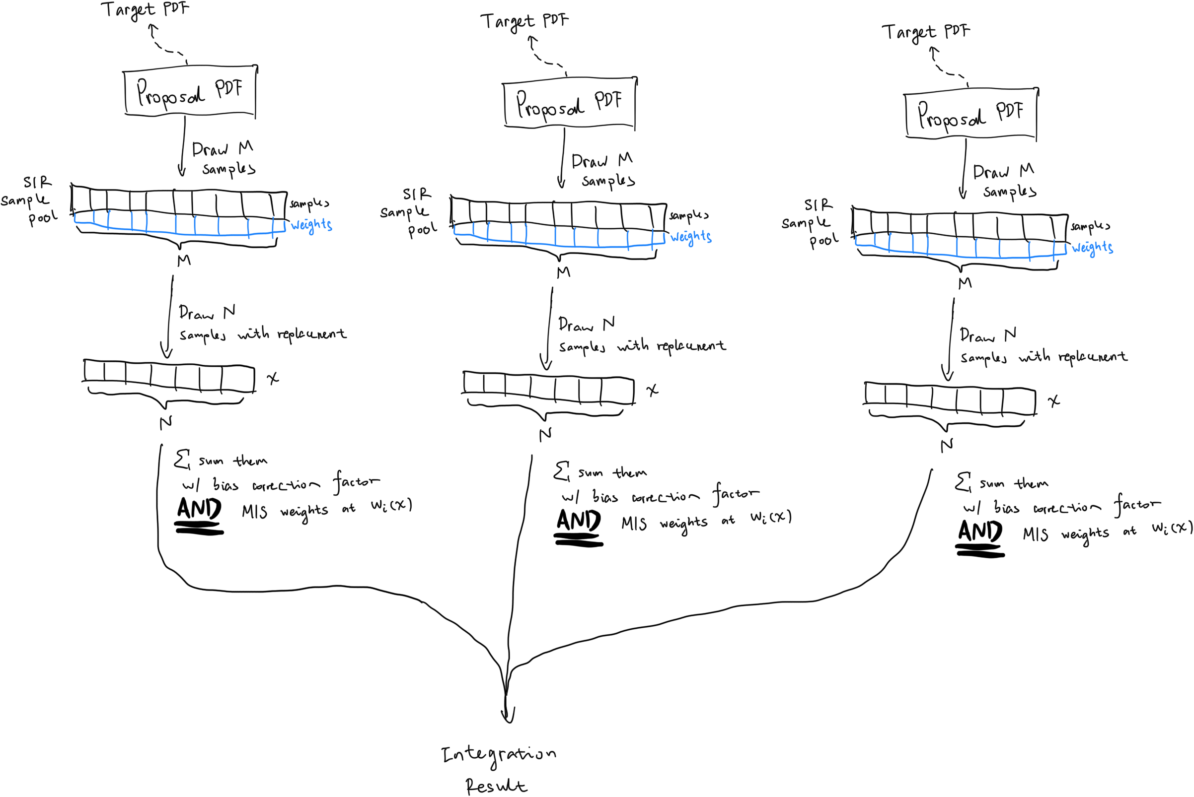
If the sketch above is too small on your screen, you can view it here.

It’s getting kind of crazy, but stay with me. Another way of combining RIS with MIS is that we can draw from multiple proposal PDFs forming the initial sample pool of M. We can then evaluate the integration result using RIS. One small modification is needed: we need to update the SIR weights to

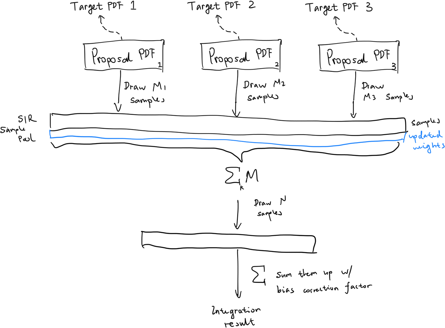
Here’s the original image.

Weighted Reservoir Sampling (WRS)

In the example presented above, even if the RIS has a sample size of \(N=1\), since we need to sample that from the SIR sample pool, we still need to store the whole SIR sample array, which has a storage size of M, so that’s not good. But do we really need that?

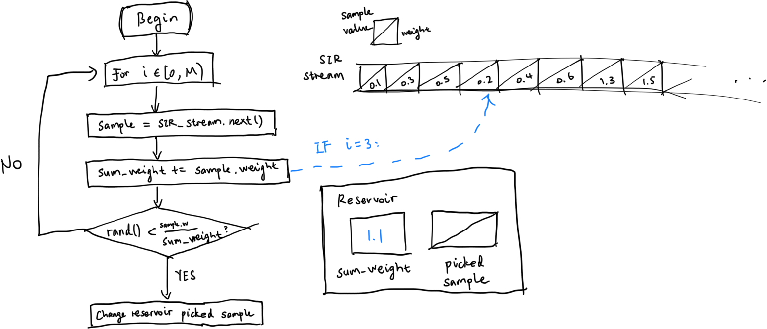
Here’s when the Weighted Reservoir Sampling (WRS) comes into play. It basically looks like this:

struct Reservoir
{
    Sample picked;
    float sum_weights;
};

//
// Update the reservoir;
// sum_weights will be updated to the total number of weights seen so far.
// If the randomly generated number is less than the normalized weight 
// for current sample, then we pick the sample.
//
void update(Reservoir &r, Sample s)
{
    r.sum_weights += s.weight;
    if (random() < s.weight / r.sum_weights)
    {
        r.picked = s;
    }
}

//
// Reservoir sample a stream of samples, for M times.
//
void reservoir_sampling(Reservoir &r, Stream<Sample> &s, int M)
{
    for (int i = 0; i < M; i++)
    {
        r.update(s.next());
    }
}

Now, this algorithm is very useful because it effectively reduces the storage requirement to \(O(1)\), because we no longer need an array to maintain the M samples we take using the SIR method anymore.

Naive ReSTIR DI

Finally, we have gathered all prerequisite knowledge for ReSTIR, short for Reservoir-based Spatio-Temporal Importance Resampling. The basic idea is just that - combining RIS with WRS:

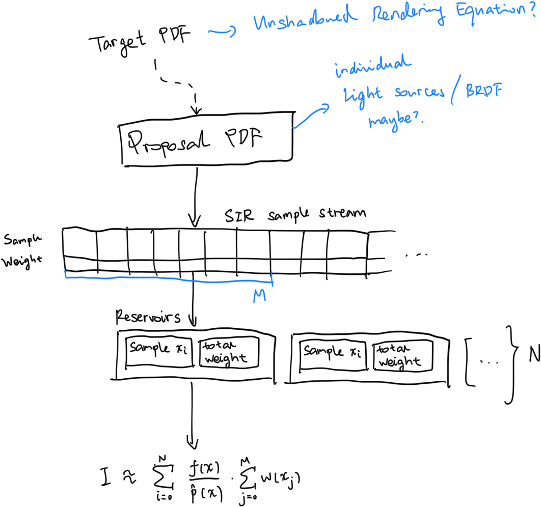
According to the paper, it states “We generate samples uniformly over the area of emitters and use the unshadowed path contribution \(\hat{p}(x) = \rho(x) L_e(x) G(x)\) as the target distribution, only tracing shadow rays for the N surviving RIS samples.” In other words, the SIR sample stream generates samples over the hemisphere where direct lighting from emitters could hit sample point; then WRS is used to pick the One True Sample (or Multiple True Samples), and integration is done over it. Since we don’t need to trace shadow rays, the SIR samples are relatively cheap to come by, and there’s little to nothing to integrate. Therefore, the whole process is very quick, and the integrated result is kind of correct.

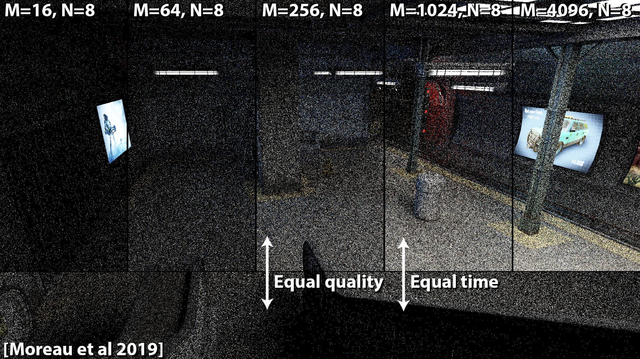
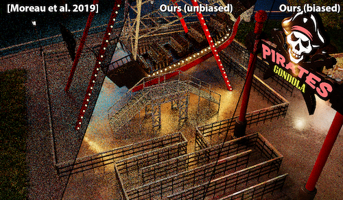
As we can see here, compared to Moreau et al.’s importance sampling algorithm, RIS with WRS can already render the subway scene either faster under the same quality, or, better quality in the same time.

ReSTIR DI then takes it one step further and states that obviously when two shading pixels are very close to each other, their lighting contributions must be very similar as well, so we can actually reuse that result. Here, ReSTIR exploits a very cool feature of WRS: the WRS procedure can be recursive. As in, we can do weighted reservoir sampling on reservoirs. Since reservoirs also hold a sample value and a weight, which is the requirement of a WRS sample, reservoirs themselves can act as a sample as well. So, by sampling neighbor’s reservoir and current shading pixel’s own reservoir, we may obtain a better result when the neighbor’s reservoir holds a better sample.

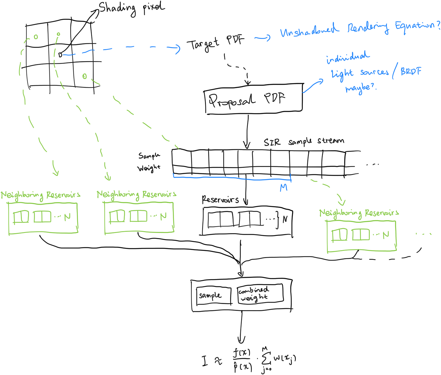
Because we are importance sampling the unshadowed Rendering Equation (with light emitters being proposal PDFs,) sometimes we may generate rays that hits an obstacle on the way to the light source. Those are bad samples, and we discard the reservoir here, so they do not partake in the spatial reusage.

If we are already reusing spatial neighbors anyway, why not take it one step further (again) and reuse temporal information as well? Like Temporal Anti-Aliasing (TAA)? So let’s do it! Let the prior frame be part of the contribution as well.

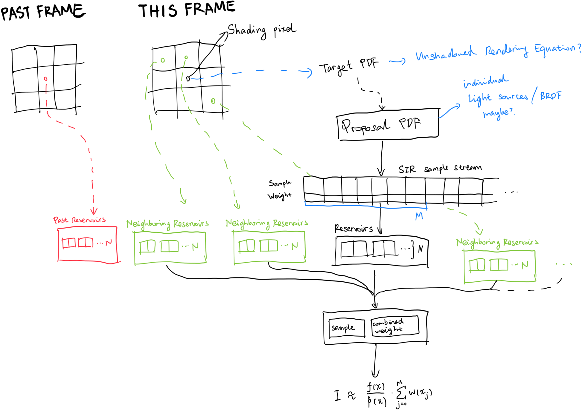
Obviously bad, occluded samples from the past frame need to be discarded as well.

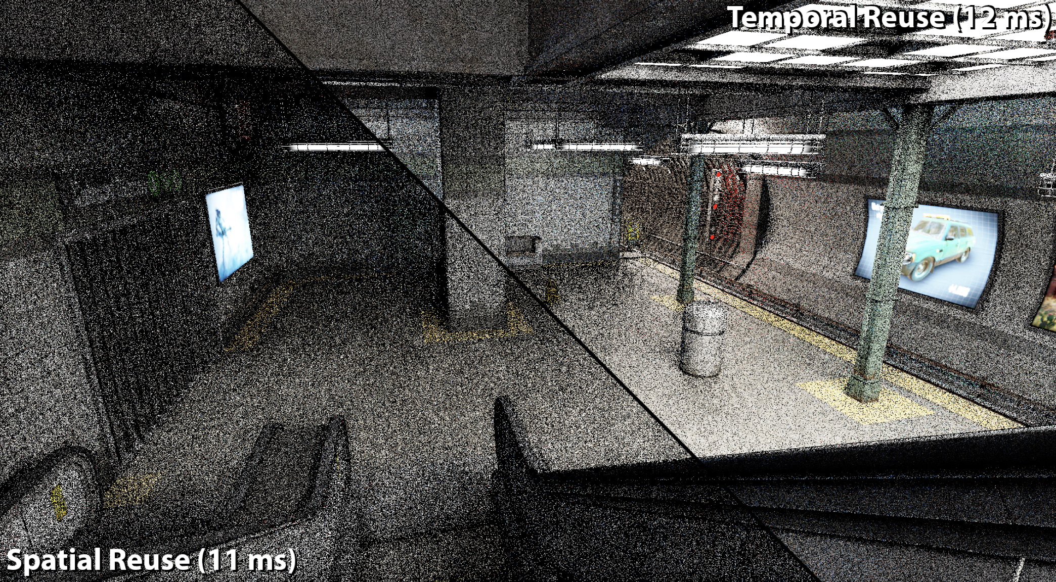
Below is a comparison between with/without temporal reuse. As we can clearly see, the render has been greatly enhanced, with almost no extra computational cost.

So yeah, that’s ReSTIR DI, in a (very big) nutshell. The end. Thanks for reading. Bye!

Bias

Except it isn’t. Why? Because renders done in this way is actually biased; spatial & temporal reuse means samples are drawn from different pixels, but each pixel have a different integration domain, and reusing that may introduce bias. However, since we are just understanding the basics of ReSTIR here, it’s kinda out of the the scope of what we are discussing here today (I also maybe didn’t read that far.) If you are interested, you can check out some reference articles. All of them are of great help during my study.

References

• Understanding The Math Behind ReStir DI | A Graphics Guy’s Note: very very helpful article. Way more in depth than this one, so please check it out.
• Monte Carlo Integral with Multiple Importance Sampling | A Graphics Guy’s Note: an article that introduces MIS thoroughly.
• Chapter 9: Multiple Importance Sampling: chapter 9 of Veach’s thesis.
• Spatiotemporal reservoir resampling for real-time ray tracing with dynamic direct lighting: the original ReSTIR paper released by NVIDIA.
• ReSTIR GI: Path Resampling for Real-Time Path Tracing: a variant of ReSTIR.
• Generalized Resampled Importance Sampling: Foundations of ReSTIR (also known as ReSTIR PT): another variant of ReSTIR.
• Volumetric ReSTIR: yet another variant of ReSTIR.
• Importance Resampling for Global Illumination: the original RIS paper by Talbot.

Comments

A valid, non-empty username is required.

Comment