Computational resources are valuable, even with that sweet, sweet GPU. Sometimes, GI at 60fps per second is simply not attainable, especially when its 2000 or something, when computational resources are way more scarce. Now, what if we time travel back to the past, and we have to render a complex scene, at 60 frames per second, with one catch that the whole scene is diffuse? This is where spherical harmonics comes in handy.

The Paper

Proposed by Peter-Pike Sloan et al., Precomputed Radiance Transfer (PRT) is a real time, global illumination rendering technique using spherical harmonics. Now, I know what you are asking. Why learn some age-old technique when the GPUs right now have real time raytracing built right into their core? If not for the sake of learning, maybe the fact that it is still very much used in modern day game engines under the name Light Probes can motivate you. So, let’s dive right in!

The Question

• How would a PBR diffuse scene look like in an environment map
• Can we render it in real time?

The first is easily solvable in raytracing or raymarching, since we are sending rays everywhere and it’s bound to sample the environment map in some point. The same cannot be said for rasterization, which real time rendering uses. To understand what an environment map is, we can look at this video illustration made by Keenan Crane (or his students) (the project website is sadly offline now so I can just link to the course website):

Click to play the video. In short, an environment map is a 2D texture $f$, wrapped onto a sphere, so that it can be sampled using spherical parameter $f(\theta ,\varphi )$.

In rasterization, shading a pixel using an environment map as lighting means calculating how light interacts with every pixel on the environment map, which could take up a lot of time. To understand how this works, or why do we need spherical harmonics to begin with, we need to take a look at the Rendering Equation.

The Rendering Equation

$$L_o(p,{\omega }_o)=L_e(p,{\omega }_o)+{\int }_{S^2}f(p,{\omega }_o,{\omega }_i)L_i(p,{\omega }_i)V(p,p^{\prime })G(p,p^{\prime })|\cos {\theta }_i|d{\omega }_i$$

Since this is a recursive algorithm, evaluating the $L_o(p,{\omega }_o)$ will be very costly during runtime. We need to find a way to perform the precalculation, and store the lighting result somehow. Render baking might work, but the lighting breaks if the scene is dynamic, i.e. there is an object transformation, such as translation or rotation. Even though light map means the light is coming from infinitely far away, an object moving doesn’t really affect the lighting, rotation can still break it.

Putting those thoughts aside, let’s focus on the Rendering Equation now. In this rendering equation, $G(p,p^{\prime })$ is the geometry albedo term; $V(p,p^{\prime })$ stands for visibility test, so if current sample point $p$ can reach the point where this ray comes from $p^{\prime }$ unobstructed, then $V(p,p^{\prime })$ returns 1; otherwise it returns 0. The biggest problem lies in the ${\int }_{S^2}$ symbol, which is a hemispherical integration, and can take up a lot of time; and the $L_i(p,{\omega }_i)$, which is a recursive term, and if the integration makes solving the RE slow, this makes solving RE real time infeasible. So, let’s start simplifying it!

To start it all off, we are going to get rid of the recursive term. If the light never bounces off other objects, and comes straight from the environment map, then there is no recursive term to speak of:

$$L_o(p,{\omega }_o)=L_e(p,{\omega }_o)+{\int }_{S^2}f(p,{\omega }_o,{\omega }_i)L_{ϵ}(p,{\omega }_i)V(p,p^{\prime })G(p,p^{\prime })|\cos {\theta }_i|d{\omega }_i$$

Now, if we combine the scattering function, visibility test, geometry albedo & the cosine term into one function, which we call transport function $T(p,p^{\prime },{\omega }_i,{\omega }_o)$, the rendering equation can be greatly simplified (on paper):

$$L_o(p,{\omega }_o)=L_e(p,{\omega }_o)+{\int }_{S^2}{L}_{ϵ}(p,{\omega }_i)T(p,p^{\prime },{\omega }_i,{\omega }_o)d{\omega }_i$$

If we assume that the only light emitter in the scene is the environment map, then the $L_e(p,{\omega }_o)$ term can be removed. Also, in a Lambertian diffuse scene, the scattering function is agnostic to the outgoing ray direction (isotropic); as a result, the transport function can be simplified again:

$$L_o(p,{\omega }_o)={\int }_{S^2}{L}_{ϵ}(p,{\omega }_i)T(p,{\omega }_i)d{\omega }_i$$

In conclusion, if we want to calculate the scene radiance of diffuse surfaces, ignoring interreflections & light emitting objects in scene, this is the final end simplification result. However, the hemispherical integration is still there, and it slows down performance. We need to find a way to get rid of it as well.

Getting Rid of the ${\int }_{S^2}$

Take a look at basis vectors and its definition: in an N-dimensional space, N non-colinear vectors can represent all coordinates in said space with a weighted sum:

What we are most interested in however, are orthonormal basis vectors, which means those vectors have a length of 1, and they are all perpendicular to each other, i.e. $⟨a,b⟩=0$ if $a!=b$.

With a set of orthonormal basis vectors, we can propose a projection procedure, which projects any point $p$ in canonical space to the space defined by the set of orthonormal basis vectors $S$:

$$a=\left[\begin{array}{c}⟨S_1,p⟩\\ ⟨S_2,p⟩\\ ⟨S_3,p⟩\\ \dots \end{array}\right]$$

$⟨x,y⟩$ denotes a dot product between vectors. The result is a coefficient vector, which then can be reconstructed back to the canonical space:

$$p=\sum _{i=1}^n{a}_i{S}_i$$

Now, to get an intuition about what we are going to do next, imagine the vector dimension goes up. As it goes up and up, there are more and more components in a vector, and eventually, as the dimensionality approaches infinite, dot operation becomes the sum of the products of infinite elements. In math terms, it becomes this:

$$⟨f,g⟩={\int }_{-\mathrm{\infty }}^{+\mathrm{\infty }}f(x)g(x)dx$$

Since infinite dimension vector is basically a function, we denote it as such. Infinite vector length (function length) is thus defined as

$$||f||=\sqrt{{\int }_{-\mathrm{\infty }}^{+\mathrm{\infty }}{f}^2(x)dx}$$

As a result, vector operations on functions make sense - it also has a name, Vector Calculus, and you can check it out on Wikipedia. In fact, function operators on vectors also make sense, such as the Laplace operator. But we are not covering it today.

Take a look back at the simplified rendering equation. If we can somehow perform a projection on both $L_{ϵ}$ and $T$ and map them onto some function space with, say, an infinite series of orthonormal functions ${\beta }_1,{\beta }_2,\dots ,{\beta }_n$, which transforms both functions into a coefficient vector $l$ and $t$, then during execution, we can restore them by performing the reconstruction. Although it feels like some needlessly complex extra steps, this is when magic happens. Because when we plug them back into our simplified Rendering Equation, this is what we get:

$$\begin{array}{rl}{L}_o(p,{\omega }_o)& ={\int }_{S^2}{L}_{ϵ}(p,{\omega }_i)T(p,{\omega }_i)d{\omega }_i\\ & ={\int }_{S^2}\sum _{j=1}^n(l_j{\beta }_j({\omega }_i))T(p,{\omega }_i)d{\omega }_i\\ & =\sum _{j=1}^n{l}_j{\int }_{S^2}{\beta }_j({\omega }_i)T(p,{\omega }_i)d{\omega }_i\\ & =\sum _{j=1}^n{l}_j{t}_j(p)\end{array}$$

We have successfully gotten rid of the integration symbol, and the Rendering Equation devolves into a simple dot operation between two different vectors. Dot operation is, of course, very trivial and quick and definitely can be evaluated real time when the vector dimension is low; in order to obtain the projected vectors however, we need to perform precalculation on both the environment map and all vertices on the scene ($p$ is still inside the final simplified Render Equation as a parameter.) This is going to be really slow, but it doesn’t matter because users won’t be able feel it - we can perform the precalculation ourselves, way before the application is run. We can then embed the vectors inside the vertex somehow.

The only problem left is to find a set of orthonormal functions defined on spherical space.

Associated Legendre Polynomials (ALP)

To understand what is spherical harmonics, we have to take a look at the Associated Legendre Polynomials first. ALP is defined as follows, and can be evaluated incrementally:

$$P_l^m:=\{\begin{array}{l}x(2m+1)P_m^m,l=m+1\\ (-1m{)}^m(2m-1)!!(1-x^2{)}^{\frac{m}{2}},l=m\\ \frac{x(2l-1)P_{l-1}^m-(l+m-1)P_{l-2}^m}{l-m},\text{otherwise}\end{array}$$

$m$ needs to be within $[-l,l]$ for any given layer $l$. !! stands for a double factorial:

int double_factorial(int n)
{
    int ret = 1;
    for (int i = n; i >= 1; i -= 2)
    {
        ret *= i;
    }
    return ret;
}

It looks crazy, I know. But all of those doesn’t matter. What matters is the properties ALP offers:

1. It’s length between $[-1,1]$ is 1 (Function length is defined as $\sqrt{{\int }_{-1}^1{f}^2(x)dx}$)
2. Orthonormal between different $l$s, i.e. $⟨P_l^m,P_{l+1}^m⟩=0$
3. Orthonormal between different $m$s within the same $l$, i.e. $⟨P_l^m,P_l^{m+1}⟩=0$

This is how it looks like when plotted:

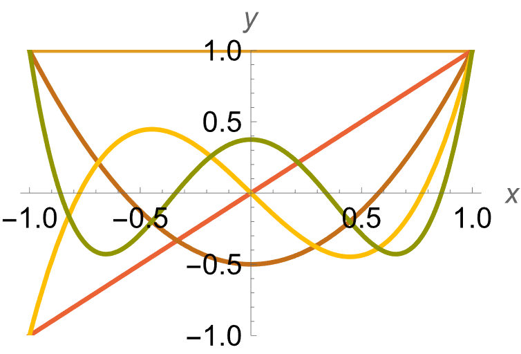
This is very cool, an infinite series of orthonormal functions, defined between $[-1,1]$. But it isn’t defined on spherical space. Enter spherical harmonics.

Spherical Harmonics

Spherical harmonics are orthonormal functions defined over a unit sphere, which at its core, is ALP with extra steps:

$$y_l^m:=\{\begin{array}{l}\sqrt{2}{K}_l^m\cos (m\varphi )P_l^m(\cos (\theta )),m>0\\ \sqrt{2}{K}_l^m\sin (-m\varphi )P_l^{-m}(\cos (\theta )),m<0\\ K_l^0{P}_l^0(\cos (\theta )),m=0\end{array}$$

In which $K_l^m$ is defined as

$$K_l^m:=\sqrt{\frac{2l+1}{4\pi }\frac{(l-|m|)!}{(l+|m|)!}}$$

This is how spherical harmonics looks like:

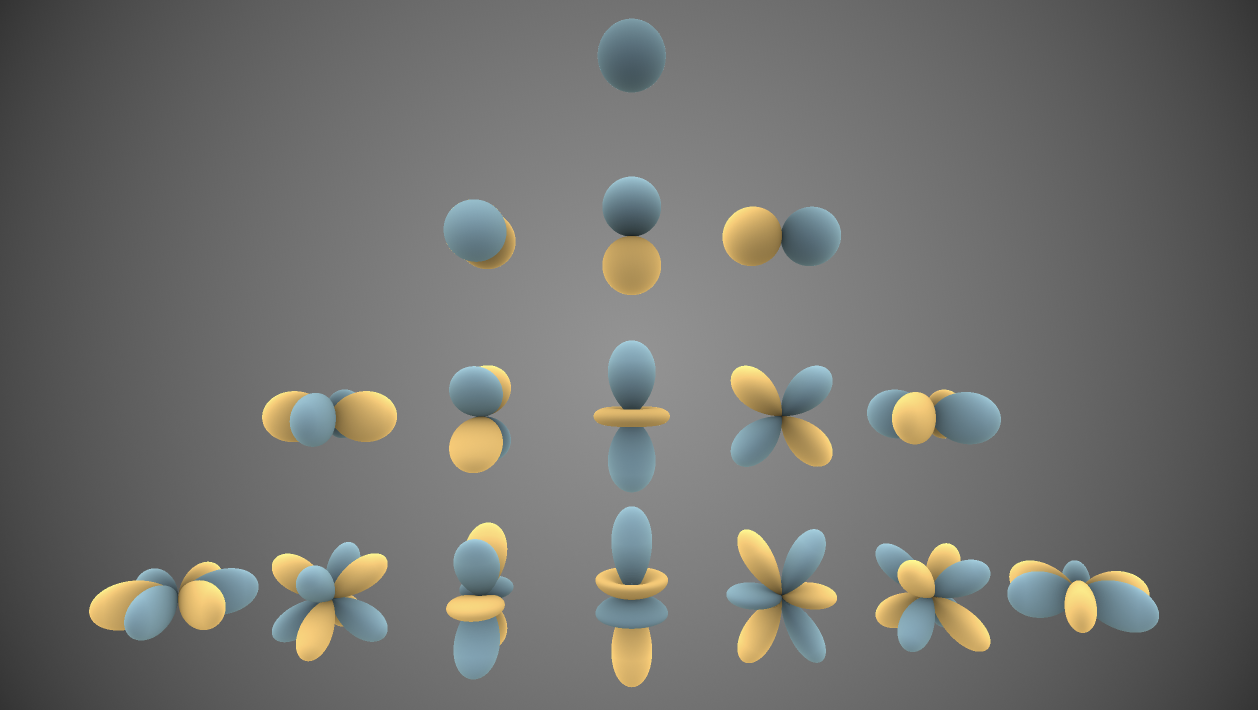
Inigo Quilez wrote a spherical harmonics shader on Shadertoy, which renders the image above using the solved version of spherical harmonics. I have written a SH solver using GLSL as well, but it doesn’t look as fancy. Still though, you can check it out!

$l$ is called the “band index” of an SH function, and since $m\in [-l,l]$ for its respective band index, the result is a pyramid-like shape. It’s also customary to index SH using a 1D vector: $i:=l(l+1)+m$. In this way, we can index the SH function using $y_i$.

Projection & Reconstruction

With the correct orthonormal function series in hand, we can now perform the projection to the scene. First, we perform projection to the environment map, up to the first $n$ band:

$$l=\left[\begin{array}{c}⟨y_0,L_{ϵ}⟩\\ ⟨y_1,L_{ϵ}⟩\\ ⟨y_2,L_{ϵ}⟩\\ \dots \\ ⟨y_n,L_{ϵ}⟩\end{array}\right]$$

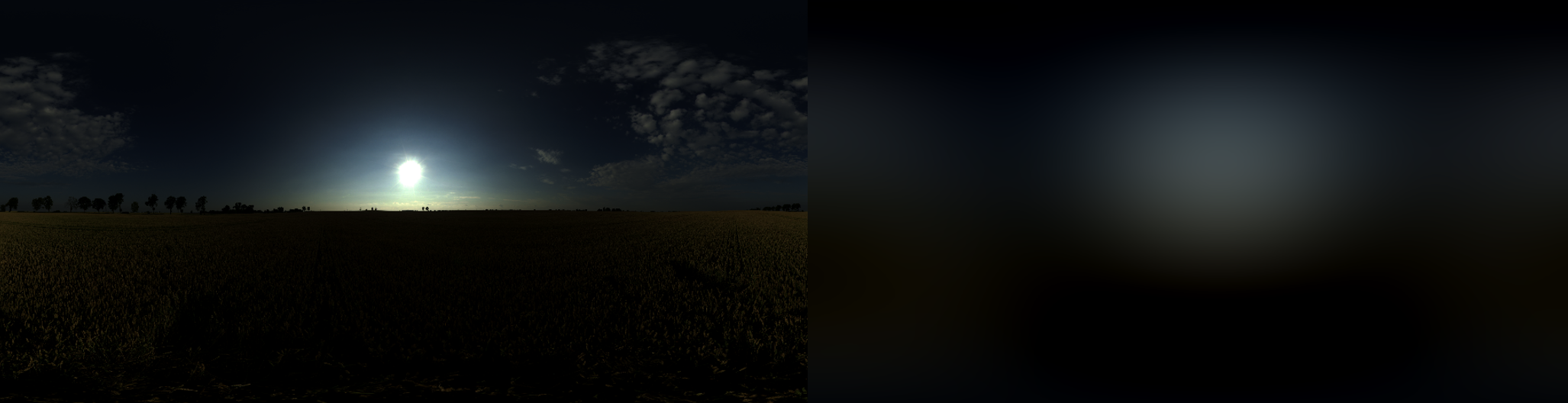
The projected result, after reconstructed, is a blurred version of the environment map - that is to be expected, as $n$ is not infinite, and as a result, cannot accurately represent the environment map itself.

The blur won’t affect the end result (that much,) since the whole scene is diffuse to begin with, and information is going to be lost anyway. If a specular object exists in the scene, the reflection will be very blurred, and the loss of information will become very apparent.

Here’s a comparison, with the left image being the original environment map and the right one being the reconstructed version:

Then, we perform projection vertex-wise to the scene:

$$t=\left[\begin{array}{c}⟨y_0,T(p)⟩\\ ⟨y_1,T(p)⟩\\ ⟨y_2,T(p)⟩\\ \dots \\ ⟨y_n,T(p)⟩\end{array}\right]$$

What can be projected per vertex? This highly depends on what we want to project. In my implementation (which is given below), I have only projected the cosine term $|\cos {\theta }_i|$, ignoring all other terms in the transport function. But theoretically, everything within the transport function can be projected, including visibility test, geometry albedo, etc.

During rendering, a simple dot operation in shader is suffice:

in mat4 shCoeffs;
uniform vec3 scene[16];
out vec4 color;

void main() {
    vec3 objColor = vec3(1.0);
    vec3 r = vec3(0.0);

    for (int i = 0; i < 4; i++) {
        for (int j = 0; j < 4; j++) {
            r += (objColor * shCoeffs[i][j]) * scene[i * 4 + j];
        }
    }
    color = vec4(r, 1.0);
}

mat4 is needed here because OpenGL does not allow custom-length vertex array. As the orthonormal function series has an infinite length, we can choose the first $n$ bands to project. The reconstructed result gets more and more accurate as $n$ increases. Here we picked the first 4 bands. The final reconstructed result looks like this:

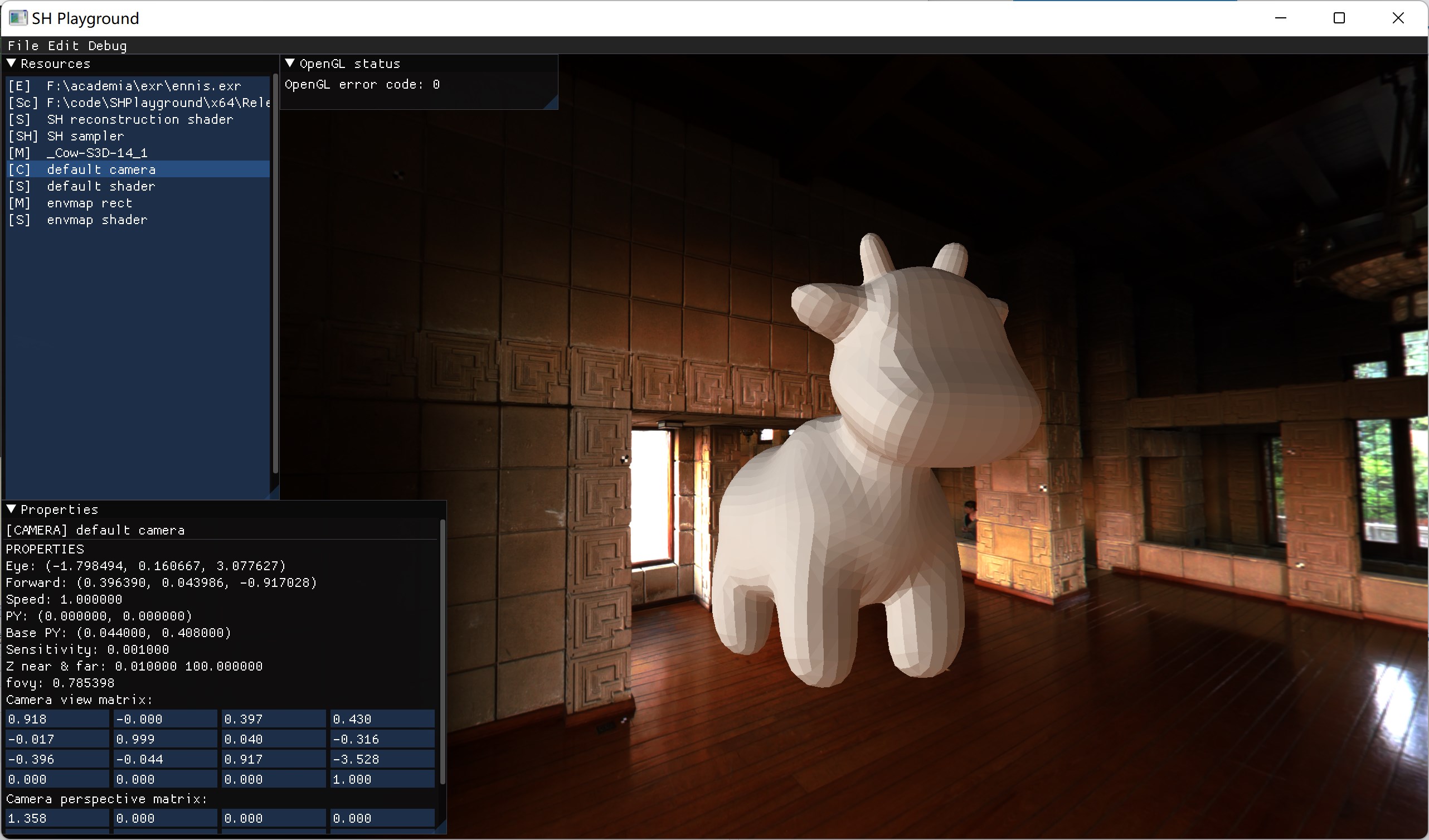
I have actually made a full-blown application for this. You can check my GitHub repo out here. Both source code and various video demos are included. Feel free to play around! It’s CUDA accelerated, so you will need an NVIDIA GPU with CUDA architecture support and CUDA toolkit installed.

Caveats

That’s it! We have successfully rendered a PBR scene (without interreflection) in real time, 60fps. However, we have traded off quite a few things during this feat:

• The scene radiance and the transport function should preferrably be low frequency
• High frequency function approximation requires higher band projection, which should be avoided ($n^2$ growth)
• Can only work with diffuse surface with no occlusions (for now)

Further Readings

There are a lot more to discuss. For example, spherical harmonic-projected coefficient vectors can actually be rotated due to its property. The original paper actually implemented self-occlusion, but I didn’t get that far. There is also neighborhood transfer (so interreflection,) and volumetric transfer (clouds!). Here are some more papers to check out, if you are interested, or if you are still confused after reading this:

• Precomputed Radiance Transfer for Real-Time Rendering in Dyanmic, Low-Frequency Lighting Environments: the original method proposed by Peter Pike Sloan et al.
• Spherical Harmonic Lighting: The Gritty Details: another article explaining spherical harmonics. It was very helpful during my research.
• A Gentle Introduction to Precomputed Radiance Transfer: article explaining PRT & SH. Also pretty helpful.
• Sparse Zonal Harmonic Factorization for Efficient SH Rotation: a zonal harmonic factorization method proposed by Derek Nowrouzezahrai et al. I am very stumped when reading this, but I think it’s pretty cool, so I am putting it here.

Comments

A valid, non-empty username is required.

Comment