I have always been amazed by Inigo Quilez’s Fruxis shader. The fruits, the lighting, it’s just perfect. The source code however, can be obscure and kind of hard to understand. So today, we are going to deconstruct & reconstruct the shader, with the exact replica of Fruxis as our end result. Let’s begin!

Bare Bones Raymarching

In order to reproduce the fruits from the shader, we have to start with a bare bones raymarching framework. If you are unfamiliar with what raymarching means, I highly recommend you check out this article written by Jamie Wong. I will list the raymarching skeleton code we are going to use below without much explanation, so give it a read first if you want.

//
// Fruxis, reconstructed - by 42yeah
//

float ball(vec3 p, vec3 center, float r)
{
    return length(p - center) - r;
}

// Maps to the closest point in scene.
// The whole scene is defined in map() function.
// Components: x: closest distance to surface
//             y: closest surface ID (so that we can shade it)
vec2 map(vec3 p)
{
    // Demo ball
    return vec2(ball(p, vec3(0.0), 1.0), 0.5);
}

vec2 march(vec3 ro, vec3 rd)
{
    int steps = 100;
    float dist = 0.01;
    
    for (int i = 0; i < steps; i++)
    {
        vec2 info = map(ro + dist * rd);
        if (info.x < 0.001)
        {
            return info;
        }
        dist += info.x;
    }
    return vec2(1.0, -1.0);
}

// Shade the particular point of the scene, according to shading informations
// given in the function parameters. We are going to determine the object color 
// at point p here as we add more and more fruits.
vec3 getColor(vec2 info, vec3 p)
{
    float id = info.y;
    if (id < 0.0)
    {
        // Shade sky
        return vec3(0.7, 0.9, 1.0);
    }
    else if (id > 0.0 && id < 1.0)
    {
        // The demo ball
        return vec3(1.0, 0.5, 0.0);
    }
    // Unknown
    return vec3(1.0, 0.0, 1.0);
}

void mainImage(out vec4 fragColor, in vec2 fragCoord)
{
    vec2 uv = fragCoord.xy / iResolution.xy;
    uv = uv * 2.0 - 1.0;
    
    vec3 ro = vec3(0.0, 0.0, 3.0);
    vec3 center = vec3(0.0, 0.0, 0.0);
    vec3 front = normalize(center - ro);
    vec3 right = normalize(cross(front, vec3(0.0, 1.0, 0.0)));
    vec3 up = normalize(cross(right, front));
    mat3 lookAt = mat3(right, up, front);
    vec3 rd = lookAt * normalize(vec3(uv, 1.8));
    
    vec2 info = march(ro, rd);
    vec3 color = getColor(info, ro + info.x * rd);
    
    color = pow(clamp(color, 0.0, 1.0), vec3(0.4545));
    
    fragColor = vec4(color, 1.0);
}

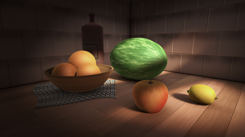
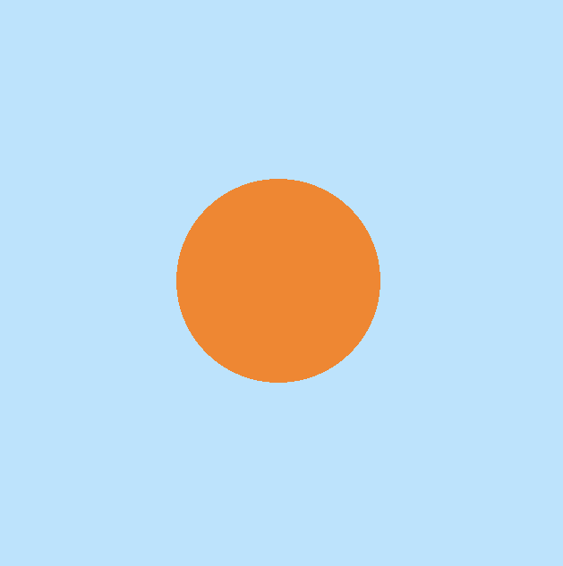
This is how it looks like: an unshaded, orange sphere in the center. Nothing much is going on, but we have laid solid foundation for what we need to do next.

Defining Geometries in the Scene

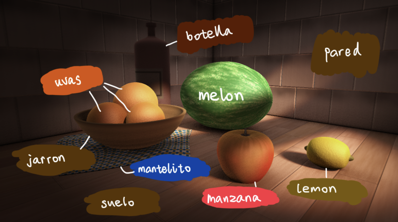
Next up, we need to define the SDF geometries used in the scene one by one. Since the name of the fruits in the original Fruxis shader are written in Spanish, we are going to honor that and write our fruit names in Spanish as well. (This also makes it easier to compare our shader with Inigo Quilez’s.) First up, here’s a exhasutive list of geometries in iq’s original shader, coupled with their respective Spanish names:

• Floor - suelo
• Wall - pared
• Melon - melon
• Apple - manzana
• Oranges - uvas (“grapes” in English)
• Lemon - lemon
• Bowl - jarron
• Doily - mantelito
• Bottle - botella

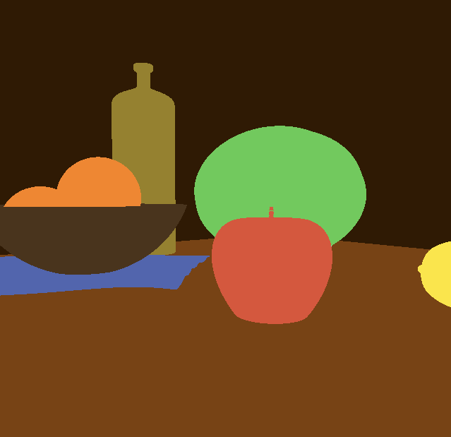
A labelled image is presented below:

Let’s start defining them one by one.

Floor & Walls (Suelo & Pared)

Floor & walls are easy enough to define:

float suelo(vec3 p, out vec3 uvw)
{
    uvw = p;
    return p.y;
}

float pared(vec3 p, out vec3 uvw)
{
    uvw = 4.0 * p;
    float d1 = 0.6 + p.z;
    float d2 = 0.6 + p.x;
    return min(d1, d2);
}

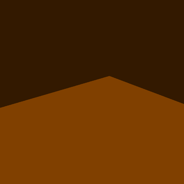
suelo returns p.y so floor is defined at \(y=0\); pared are defined so that walls are parallel to yz plane at \(x=-0.6\) and xy plane at \(z=-0.6\). uvw is an output coordinate used at the shading & post-processing phase; we will just leave it as is for now.

After adding walls & floor, adjusting the camera position, and removing the demo ball, the scene now looks like this:

Melon

The melon is a deformed sphere, as can be seen below:

float melon(vec3 p, out vec3 uvw)
{
    vec3 c = p - vec3(0.0, 0.215, 0.0);

    vec3 q = 3.0 * c * vec3(1.0, 1.5, 1.5);
    uvw = 3.0 * c;

    float r = 1.0 - 0.007 * sin(30.0 * (-c.x + c.y - c.z));
    return 0.65 * (length(q) - r) / 3.0;
}

First, world coordinate \(p\) is transformed into melon coordinate \(c\). The position is then being further deformed in both y and z axis & turned into \(q\). Then the melon radius in the transformed coordinate is defined - although I don’t really understand the reason behind 0.007 * sin(30.0 * (-c.x + c.y - c.z)). The final signed distance function is evaluated, with further scalings done by iq.

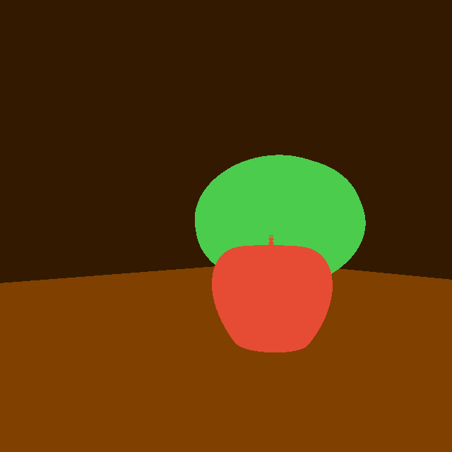
Apple (Manzana)

The apple is a deformed sphere with a stalk:

float manzana(vec3 p, out vec3 uvw)
{
    vec3 q = p - vec3(0.5, 0.1, 0.5);
    float r = length(q.xz);
    q.y += 0.05 * (1.0 - clamp(r / 0.1, 0.0, 1.0));
    q.y -= 0.03 * (1.0 - smoothstep(0.004, 0.005, r));
    uvw = 10.0 * q;
    return 0.4 * (length(10.0 * q) - 1.0) / 10.0;
}

Going over the lines one by one, here’s what we can learn from the first 4 lines:

1. Transform sample point \(p\) into apple coordinate
2. Get how far \(p\) is in the xz plane
3. Deforming the sphere body into an apple shape
4. Gives the apple an apple stalk

Oranges (uvas)

The oranges are just three spheres with varying radius:

float uvas(vec3 p, out vec3 uvw)
{
    vec3 q = p - vec3(-0.1, 0.1, 0.6);
    uvw = 10.0 * q;
    
    float d1 = length(q - vec3(-0.09, -0.1, -0.07)) - 0.12;
    float d2 = length(q - vec3(0.11, 0.05, 0.0)) - 0.09;
    float d3 = length(q - vec3(-0.07, 0.03, 0.1)) - 0.1;
    
    return min(d1, min(d2, d3));
}

The sample point \(p\) is first transformed into orange space, and three individual oranges are further transformed from the center with a slight offset. The end shape is the three spheres combined, suspended in midair. It doesn’t really matter, since we will introduce a bowl into the scene real soon, which will contain the oranges.

An interesting side note, since “uvas” means grapes in English, I think iq originally wants those to be grapes instead of oranges.

Lemon

The lemon is also a sphere, albeit severly deformed so that both ends are pointy, and have a eloganted body:

float lemon(vec3 p, out vec3 uvw)
{
    vec3 q = p - vec3(0.7, 0.06, 0.2);
    uvw = 10.0 * q;
    
    float s = 1.35; // ???
    float r = clamp(abs(q.x) / 0.077, 0.0, 1.0);
    s += 2.5 * pow(r, 24.0);
    q *= vec3(1.0, s, s);
    return 0.5 * (length(12.0 * q) - 1.0) / (12.0 * s);
}

The sample point is, of course, first transformed into a coordinate system where the lemon is situated at the center. To be frank, I don’t really understand what’s going on next. I am just going to leave it as is now, and maybe I will come back when I learn more about it.

Bowl (jarron)

The bowl is, again, a sphere. However this time, it’s a hollow sphere. It is then intersected with a plane, so that it becomes bowl-shaped:

float jarron(vec3 p, out vec3 uvw)
{
    vec3 q = p - vec3(-0.1, 0.28, 0.6);
    uvw = q;
    
    float d1 = length(q) - 1.0 / 3.5;
    d1 = abs(d1 + 0.025 / 3.5) - 0.025 / 3.5;
    
    float d2 = q.y + 0.1;
    return max(d1, d2);
}

Here’s a rough idea of what’s happening:

1. Sample point \(p\) is transformed into a space where the bowl is at the center
2. uvw is assigned
3. \(d_1\) is evaluated - it’s a sphere with a radius of \(\frac{1}{3.5}\)
4. The sphere is hollowed out with the abs operation - the bowl width is \(\frac{0.025}{3.5}\)
5. \(d_2\) is evaluated - it’s an xz plane at \(y=0.18\)
6. The plane and the sphere is intersected (max) so only the lower half of the hollow sphere is preserved

Doily (mantelito)

The doily is a deformed round box. The definition of round box, among long with a lot of other distance functions, are available on Inigo Quilez’s distfunctions page.

float mantelito(vec3 p, out vec3 uvw)
{
    vec3 q = p - vec3(-0.1, 0.001, 0.65);
    q.xz += 0.1 * vec2(
        0.7 * sin(6.0 * q.z + 2.0) + 0.3 * sin(12.0 * q.x + 5.0),
        0.7 * sin(6.0 * q.x + 0.7) + 0.3 * sin(12.0 * q.z + 3.0));
     
    const mat2 m2 = mat2(0.8, -0.6, 0.6, 0.8);   
    q.xz = m2 * q.xz;
    uvw = q;
    
    q.y -= 0.008 * (0.5 - 0.5 * sin(40.0 * q.x) * sin(5.0 * q.z));
    
    return length(max(abs(q) - vec3(0.3, 0.001, 0.3), 0.0)) - 0.0005;
}

Again, a brief idea of what the code is doing:

1. Sample point \(p\) is transformed into a space where the doily is at the center, again
2. The xz components of \(q\) is deformed (becomes wavy due to all these \(\sin\) functions)
3. The doily is rotated according to \(m_2\)
4. A miniscule offset on the y axis is applied to the doily so the doily is not perfectly flat anymore
5. Finally, the SDF distance function is evaluated

Bottle (botella)

Finally, the last object of the scene. I don’t really understand what’s going on in botella. I will try my best to explain it though.

float botella(vec3 p, out vec3 uvw)
{
    vec3 q = p - vec3(-0.35, 0.0, 0.3);
    vec2 w = vec2(length(q.xz), q.y);

    uvw = q;
    
    float r = 1.0 - 0.8 * pow(smoothstep(0.5, 0.6, q.y), 4.0);
    r += 0.1 * smoothstep(0.65, 0.66, q.y);
    r *= 1.0 - smoothstep(0.675, 0.68, q.y);
    
    // Hack
    r -= clamp(q.y - 0.67, 0.0, 1.0) * 1.9;

    return (w.x - 0.11 * r) * 0.5;
}

If you remember the original code of Fruxis, you will notice a noticable difference in my botella code and iq’s botella code. For whatever reason, using iq’s botella code results in a thin line protruding from the bottle’s cap, so I hacked around and solved the issue (in a very forced way).

As per usual, a transformation is applied to \(p\) so that the bottle is located at the center of the world. The signed distance return value is the horizontal radius (xz plane) of the bottle, subtracted with a varying \(r\). The \(r\) is evaluated according to the sampling bottle height. If we are at the neck of the bottle, then the intersected circle is smaller; if we are at the top, the intersected circle is bigger. So is the body of the bottle. A smoothstep function is used so the transition from neck to body appears smoother.

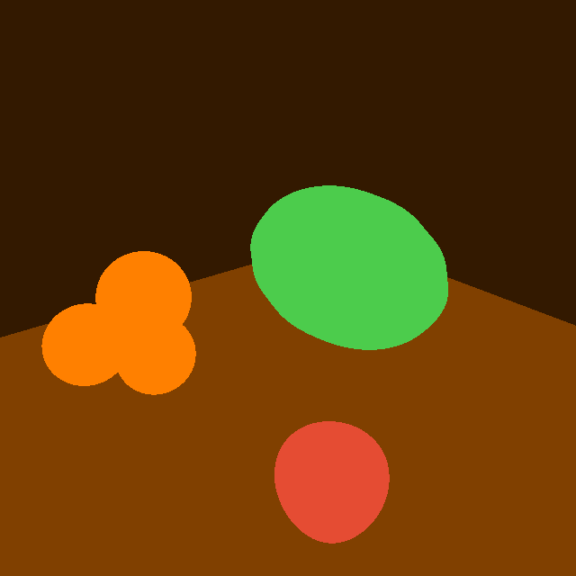
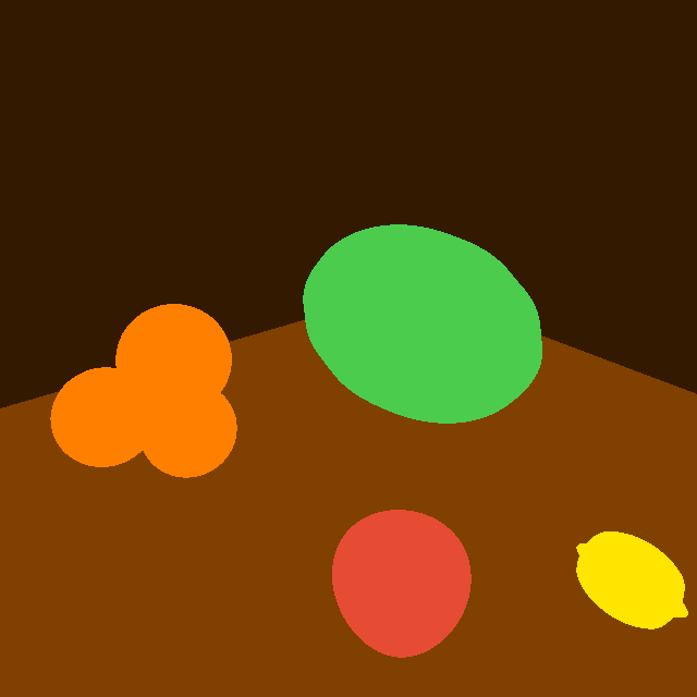
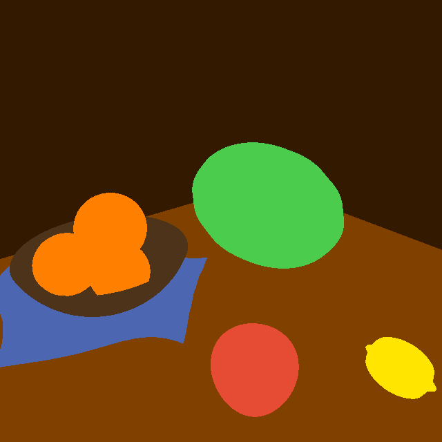
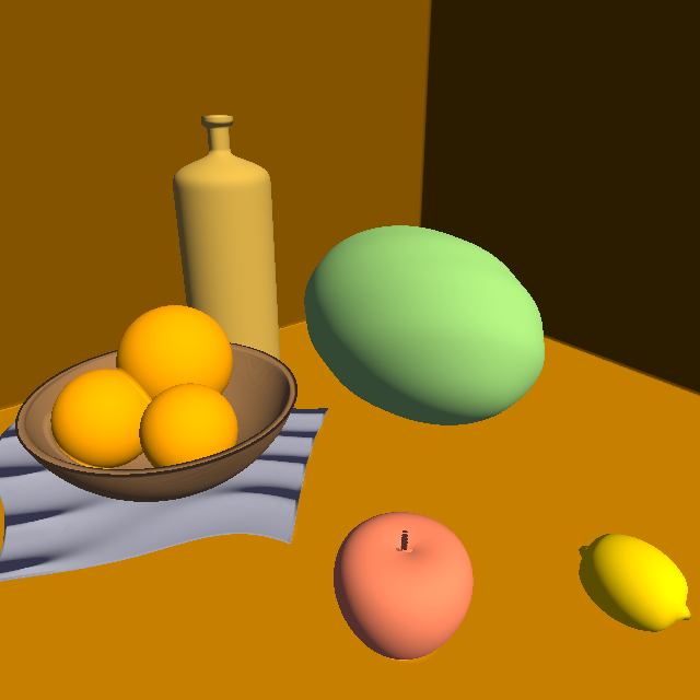
After implementing all these shapes above, if everything goes to plan, we should be able to see how the whole scene looks, without lighting. A good thing about Fruxis is, even when the whole scene is unlighted, all shapes are clearly discernible, and we can easily distinguish one geometry from the other:

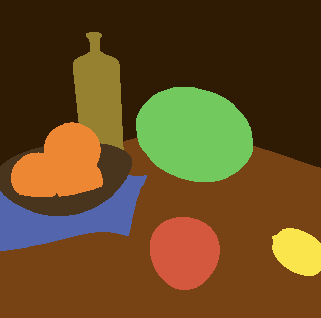
Here’s the apple stalk, seen from the side:

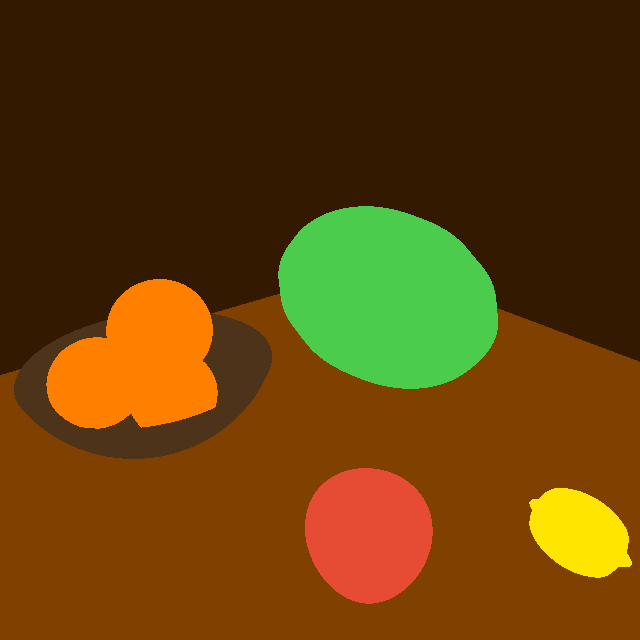
A rough color corresponding to each fruit is defined by me in the getColor function. Here’s how it looks like:

// Shade the particular point of the scene, according to shading informations
// given in the function parameters.
vec3 getColor(vec2 info, vec3 p)
{
    float id = info.y;
    if (id < 0.0)
    {
        // Shade sky
        return vec3(0.7, 0.9, 1.0);
    }
    else if (id > 0.0 && id < 1.0)
    {
        // Floor (suelo)
        return vec3(0.5, 0.25, 0.0);
    }
    else if (id > 1.0 && id < 2.0)
    {
        // Wall (pared)
        return vec3(0.2, 0.1, 0.0);
    }
    else if (id > 2.0 && id < 3.0)
    {
        // Melon
        return vec3(0.3, 0.8, 0.3);
    }
    else if (id > 3.0 && id < 4.0)
    {
        // Apple (manzana)
        return vec3(0.9, 0.3, 0.2);
    }
    else if (id > 4.0 && id < 5.0)
    {
        // Oranges (uvas)
        return vec3(1.0, 0.5, 0.0);
    }
    else if (id > 5.0 && id < 6.0)
    {
        // Lemon
        return vec3(1.0, 0.9, 0.0);
    }
    else if (id > 6.0 && id < 7.0)
    {
        // Bowl (jarron)
        return vec3(0.3, 0.2, 0.1);
    }
    else if (id > 7.0 && id < 8.0)
    {
        // Doily (mantelito)
        return vec3(0.3, 0.4, 0.7);
    }
    else if (id > 8.0 && id < 9.0)
    {
        // Bottle (botella)
        return vec3(0.6, 0.5, 0.1);
    }
    // Unknown
    return vec3(1.0, 0.0, 1.0);
}

With a mathematically well-defined, albeit unlighted scene in hand, we can start step 2: actually shading the scene.

Initial Shading

To start it off, we have to perform gamma correction first. Since without gamma correction, lighting calculations will look way off in the final result.

Performing gamma correction is easy. We simply have to raise the color to the power of \(\frac{1}{\sqrt{2.2}}\), or, in other words, around 0.4545:

color = pow(clamp(color, 0.0, 1.0), vec3(0.4545));

The colors from the original scene comes from the calcColor function, which calculates color based on given material ID, the uvw given above, and normal. This function should correspond to our getColor function, which does the same thing. In order for that to work, we have to implement a getNormal first, a standard practice in raymarching:

vec3 getNormal(vec3 p)
{
    vec3 uvw;
    vec2 del = vec2(0.01, 0.0);
    float val = map(p, uvw).x;

    return normalize(vec3(val - map(p - del.xyy, uvw).x,
        val - map(p - del.yxy, uvw).x,
        val - map(p - del.yyx, uvw).x));
}

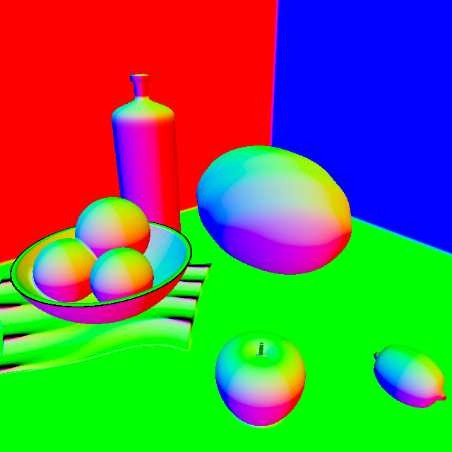
This is how the scene looks like if we shade the entire scene using its normal:

With the normal in hand, we can light the scene using a simple Phong shading model (for now), so the whole scene becomes easier to the eyes:

// ...
vec3 obj = getColor(info, uvw);
vec3 nor = getNormal(p);

// Lighting components
vec3 lightDir = normalize(vec3(1.0, 1.0, 0.0));
float ambient = 0.1;
float diffuse = max(0.0, dot(nor, lightDir));

// Lights
vec3 lin = vec3(0.0);
lin += ambient * vec3(1.0, 0.8, 1.0);
lin += diffuse * vec3(1.5, 1.1, 0.7);

vec3 color = vec3(0.0);
color += lin * obj;
color = pow(clamp(color, 0.0, 1.0), vec3(0.4545));

fragColor = vec4(color, 1.0);

Finally, dimensionality! Based on the framework here, we can implement further, more detailed lighting calculations, also based on the original Fruxis shader. Here’s an exhaustive list of lighting calculations in the original Fruxis shader:

1. Ambient Occlusion
2. Bottom light
3. Ambient lighting
4. Dome light
5. Diffuse lighting
6. Back light
7. Soft shadow
8. Fringe lighting
9. Soft specular lighting

We are going to implement all the lightings.

Attenuation

Let’s first take a look at the attenuation value, or att in iq’s shader. In Fruxis, the attenuation does not stand for light attenuation as distance goes up, but instead, makes the light acts more like a spotlight. As sample position goes higher and higher, the light gets ever so darker:

// Light position & direction
const vec3 rlight = vec3(3.62, 2.99, 0.71);
vec3 lig = normalize(rlight);
// Attenuation calculation
float att = 0.1 + 0.9 * smoothstep(0.975, 0.977, dot(normalize(rlight - p), lig));

The result? A light at \(\begin{bmatrix} 3.62 \\
2.99 \\
0.71 \end{bmatrix}\) shining at \(\begin{bmatrix} 0 \\
0 \\
0 \end{bmatrix}\). By applying att to lighting coefficients, we can achieve a spotlight-like effect. However, the effect can be very subtle. Here’s how it looks like when we set the output color to attenuation only:

Ambient Lighting

Ambient is just a constant contribution, as seen from the simple Phong lighting model above. In iq’s code, ambient is always set to 1:

// Component
float ambient = 1.0;
// ...
// Lighting contribution
lin += ambient * vec3(0.08, 0.1, 0.12) * att;

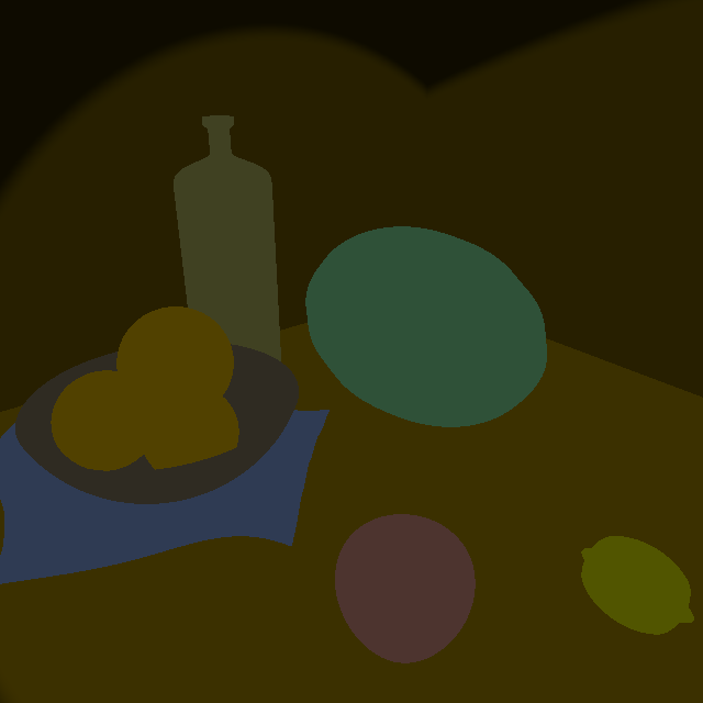
The scene lighting only by ambient lighting is simply a darkened version of the unshaded scene:

Diffuse Lighting

Next up, we are going to introduce all diffuse lights, including lights at front & back, top & bottom, and finally, fringe light.

// Components
float bfl = clamp(-nor.y * 0.8 + 0.2, 0.0, 1.0) * pow(clamp(1.0 - p.y, 0.0, 1.0), 2.0); // Bottom
float bce = clamp(nor.y * 0.8 + 0.2, 0.0, 1.0); // Dome
float dif = max(dot(nor, lig), 0.0); // Diffuse
float bac = max(dot(nor, normalize(-vec3(-lig.x, 0.0, -lig.z))), 0.0); // Back
float fre = pow(clamp(1.0 + dot(nor, rd), 0.0, 1.0), 3.0); // Fringe
// ...
// Lighting contributions
lin += bfl * vec3(0.5 + att * 0.5, 0.3, 0.1) * att;
lin += bce * vec3(0.3, 0.2, 0.2) * att;
lin += bac * vec3(0.4, 0.35, 0.3) * att;
lin += dif * vec3(2.5, 1.8, 1.3);
lin += fre * vec3(3.0, 3.0, 3.0) * att * (0.25 + 0.75 * dif);

By adding more and more lights, the scene becomes brighter and brighter, until it becomes way too bright. It is high time that we introduce shadow into the scene, which can greatly enhance realism.

Direct Lighting & Shadow

First, we need to implement a soft shadow raymarching function. You can check out iq’s article on soft shadow to learn more:

float softShadow(vec3 ro, vec3 rd, float k)
{
    float res = 1.0;
    float t = 0.001;
    vec3 trash;
    for (int i = 0; i < 64; i++)
    {
        vec2 info = map(ro + rd * t, trash);
        res = min(res, smoothstep(0.0, 1.0, k * info.x / t));
        if (res < 0.001)
        {
            break;
        }
        t += clamp(info.x, 0.01, 1.0);
    }
    return clamp(res, 0.0, 1.0);
}

The next thing is the directLighting function. Shadow is not the only thing masking the scene, there’s some sort of pre-defined mask as well, which makes the scene feels like light is filtering through the blinds. The first shadow mask is the attenuation we mentioned above, and the second mask is done by projecting the sampling point into some kind of space:

float directLighting(vec3 pos, vec3 nor)
{
    vec3 front = lig;
    vec3 right = normalize(cross(front, vec3(0.0, 1.0, 0.0)));
    vec3 up = cross(right, front);
    
    float shadowIntensity = softShadow(pos + 0.001 * nor, lig, 10.0);
    
    // attenuation
    vec3 toLight = rlight - pos;
    float att = smoothstep(0.985, 0.997, dot(normalize(toLight), lig));

    // window mask
    vec3 pp = pos - front * dot(pos, front);
    vec2 uv = vec2(dot(pp, right), dot(pp, up));
    float pat = smoothstep(-0.5, 0.5, sin(10.0 * uv.y));
    
    return pat * att * shadowIntensity;
}

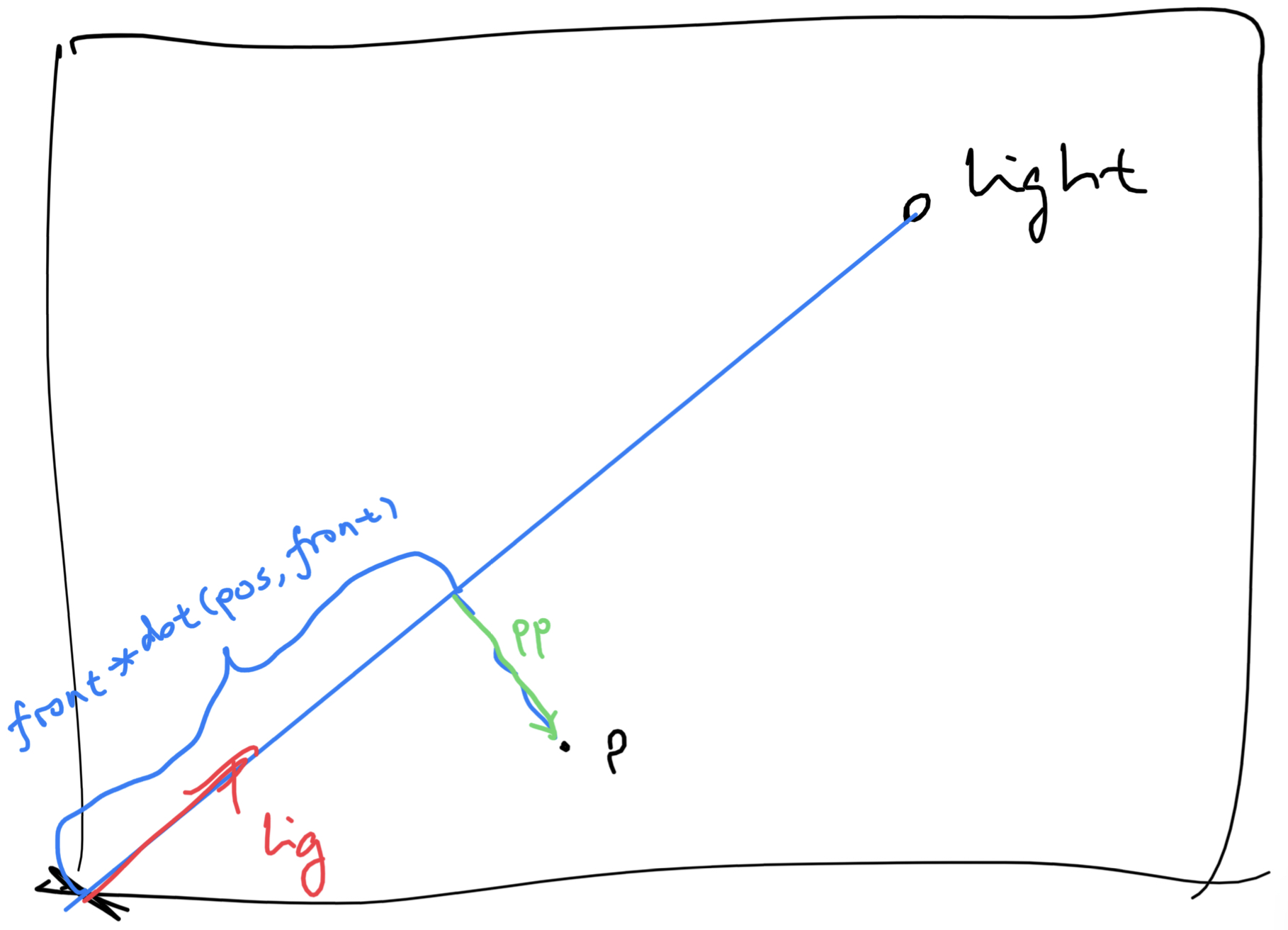
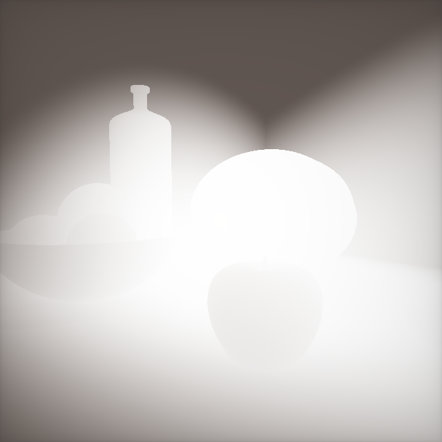
First, pp, which is a vector pointing from sample point \(p\)’s projection along the light direction to point \(p\), is evaluated. Then uv is evaluated which is basically point pp projected into a coordinate system defined by the light direction. pat the mask is evaluated by passing y component of the the projected uv coordinate into a high-frequency sin function. The mask looks like this:

And by applying the directLighting’s result to the diffuse component, here’s what we end up with:

As we can see, the realism has greatly increased.

Ambient Occlusion

To improve the realism even further, we are going to apply ambient occlusion to the scene. Raymarched scenes are good since we always have the information about the whole scene, so the ambient occlusion is actually not SSAO, but real AO performed per-pixel. You can learn more about ambient occlusion on the LearnOpenGL article. In short, ambient occlusion is achieved by sampling a bunch of random points around the sample point and determine how occluded this point is by calculating how many sample points end up in the scene geometries. This is used to simulate light bounces - if a lot of sample points are inside scene geometries, that must mean the sample point is in some sort of concave area, thus light must bounce around a lot; and as a result, should appear darker.

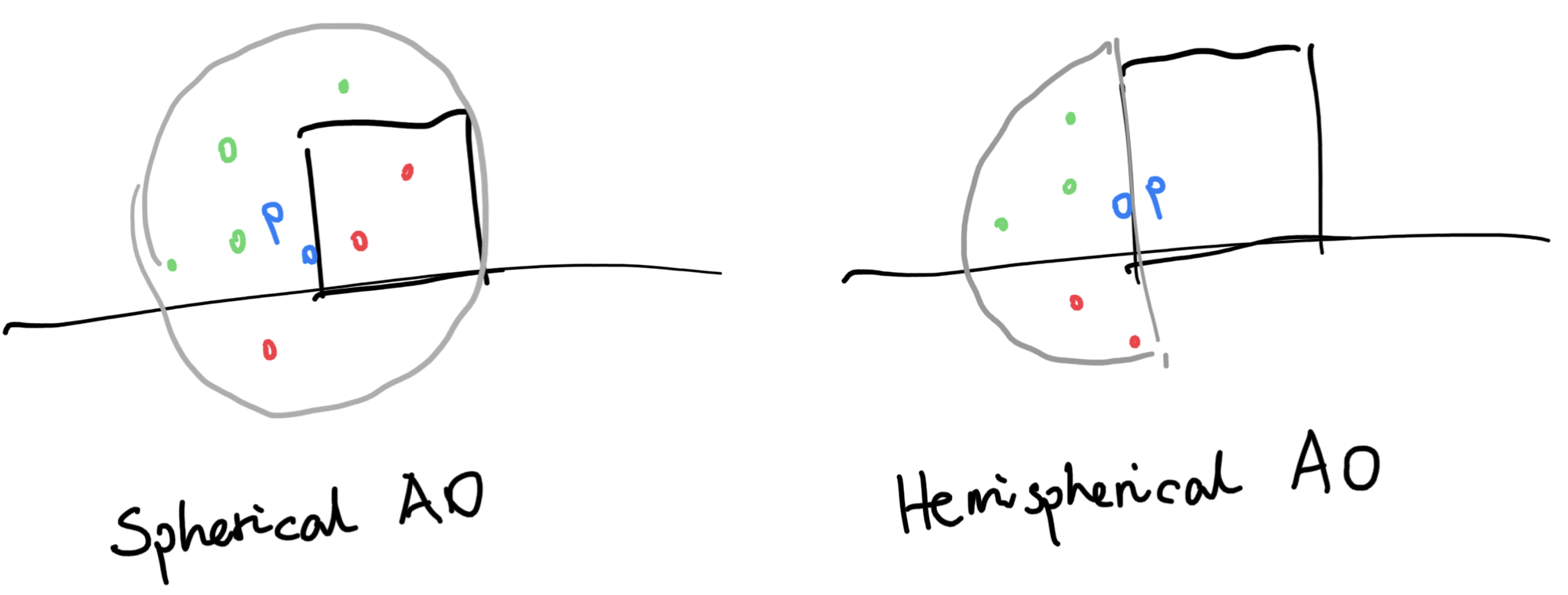
There are two kinds of AOs, namely spherical AO and hemispherical AO. In hemispherical AO, we only sample points inside the hemisphere defined by p and its normal n. Hemispherical AO has proven to be the better method over the years because spherical AO usually makes flat surfaces darker (since approximately half of the sample points will end up inside the surface.) As a result, we will be using hemispherical AO here. But to do that, we need a method to generate random points. And to generate random points, we need a hash function first.

vec3 hash3(float n)
{
    return fract(sin(vec3(n, n + 1.0, n + 2.0)) * vec3(43758.5453123, 22578.1459123, 19642.3490423));
}

This hash function is ripped straight from the original Fruxis shader. It’s just the fraction of the sine of three numbers multiplied by three very large numbers. In practice, maybe it’s not the best hash function - it tends to repeat itself; but it is very quick, and is enough for our uses.

float calcAO(vec3 p, vec3 nor, vec2 px)
{
    float off = 0.1 * dot(px, vec2(1.2, 5.3));
    float ao = 0.0;
    
    vec3 trash;
    for (int i = 0; i < 20; i++)
    {
        // Generate a random sample point (0 to 1)
        vec3 aoPos = 2.0 * hash3(float(i) * 213.47 + off);
        // Moves closer to center of the sphere
        aoPos = aoPos * aoPos * aoPos;
        // Flip points so we are now only sampling in the hemisphere
        aoPos *= sign(dot(aoPos, nor));
        // Sample those points and magnify them by 48 times
        ao += clamp(map(p + nor * 0.015 + 0.015 * aoPos, trash).x * 48.0, 0.0, 1.0);
    }
    // Calculate the average ambient occlusion value
    ao /= 20.0;
    return clamp(ao * ao, 0.0, 1.0); 
}

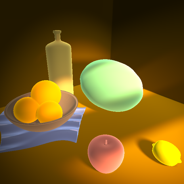
By applying the ambient occlusion result to every lighting calculations except direct diffuse lighting onto the scene, here’s what we get:

The scene is now a little bit grainy. This is due to the randomness in ambient occlusion calculation, which introduces noise. But I’d say it’s worth it.

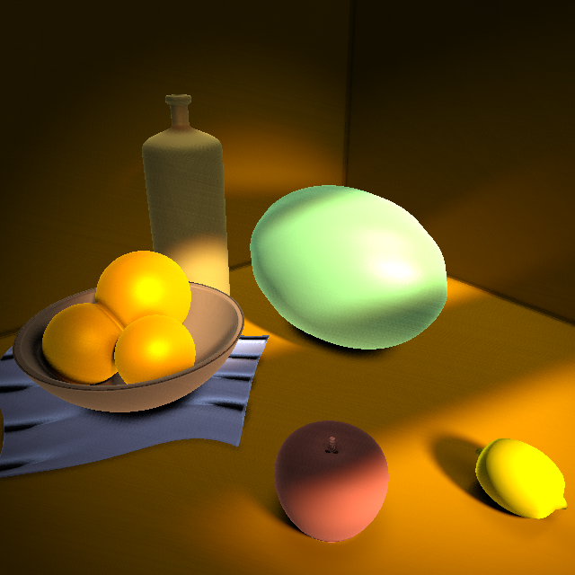
Specular Lighting

After all the diffuse lightings & shadows & stuffs, we can now add a very subtle bit of specular lighting onto the scene to make it look just a little bit better.

// Component
vec3 ref = reflect(rd, nor); 
float spe = 0.04 + 0.96 * pow(clamp(dot(ref, lig), 0.0, 1.0), 5.0);
// ...
// Lighting contribution
lin += spe * vec3(3.0, 3.0, 3.0) * occ * att * dif * sha * info.x;

My specular calculation is different from that of iq’s because I don’t really get what he was trying to do here. But the end result is very similar, so I’ll take it.

Postprocessing

With the scene almost done, now it’s time to introduce some post-processing techniques, such as adding contrast, saturation, and more. I think those are usually done under artistic direction (which I have none), but luckily I can copy those from iq’s shader code, so that’s good. We are going to apply, in order, contrast, saturation, curves, and vignetting.

// Contrast
color = color * 0.6 + 0.4 * color * color * (3.0 - 2.0 * color);
// Saturation
color = mix(color, vec3(dot(color, vec3(0.33))), 0.2);
// Curves
color = pow(color, vec3(0.85, 0.95, 1.0));
// Vignetting
vec2 q = uv * 0.5 + 0.5;
color *= 0.7 + 0.3 * pow(16.0 * q.x * q.y * (1.0 - q.x) * (1.0 - q.y), 0.15);

While contrast, saturation, and curves are both adjusting the colors, vignetting is making the center brighter and the boundaries darker, in order to achieve a cinematic effect. Here’s how it looks like, with the effects applied in order:

That’s It… For Now

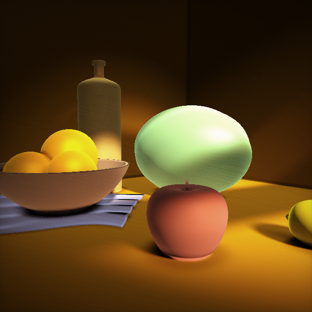
Golly gosh, That’s a lot of code snippets, and a lot of screenshots. We have re-implemented Fruxis from the ground up, even though something is still missing: the proper color of objects, and their bumps. We will solve this problem in the next part. But for now, we can imagine that we are enjoying our time in a sunny afternoon, and the sunlight is filtering through the blinds. Everything is good, and it’s a lazy, lazy day.

Lighting artifacts still exist, of course. When seen from the side, the apple is wrongly shaded: its bottom appears too bright. Hopefully we can solve that in my next blog post. The doily also appears too dark in its folds.

But yeah, we are calling it a day here. You can check out the final shader on Shadertoy. Tune in next week, as we will apply bumps to the floor, wall & oranges, as well as giving detailed texture to all of them. Hopefully, lighting artifacts present in this week will be fixed as well!

Comments

A valid, non-empty username is required.

Comment