Clouds. They are beautiful and fluffy. Take a look at Inigo Quilez’s cloud shader, and marvel at its beauty:

Today, we are going to raymarch that soft marshmellow, and we are going to jump straight into it. Let’s go!
3D Value Noise
Clouds are volumetric objects, and as a result, have no well-defined geometric shape. Rather, it’s a volume density field, a continuous n-dimensional table of values, much like what an SDF function is:
\[f(x) \rightarrow \mathbb{R}, x \in \mathbb{R}^n\]Plug whatever sample point x into the volume function, and you get a return floating point value, indicating cloud density at this specific point. But how do we get a volume that is 3D and cloud-like?
3D value noise comes to mind. Usually value noise is 2-dimensional, so it doesn’t work, however it’s pretty easy to extrapolate the underlying principle to 3-dimensional:
float valueNoise(vec3 p)
{
    vec3 u = floor(p);
    vec3 v = fract(p);
    vec3 s = smoothstep(0.0, 1.0, v);

    float a = rand(u);
    float b = rand(u + vec3(1.0, 0.0, 0.0));
    float c = rand(u + vec3(0.0, 1.0, 0.0));
    float d = rand(u + vec3(1.0, 1.0, 0.0));
    float e = rand(u + vec3(0.0, 0.0, 1.0));
    float f = rand(u + vec3(1.0, 0.0, 1.0));
    float g = rand(u + vec3(0.0, 1.0, 1.0));
    float h = rand(u + vec3(1.0, 1.0, 1.0));

    return mix(mix(mix(a, b, s.x), mix(c, d, s.x), s.y),
               mix(mix(e, f, s.x), mix(g, h, s.x), s.y),
               s.z);
}
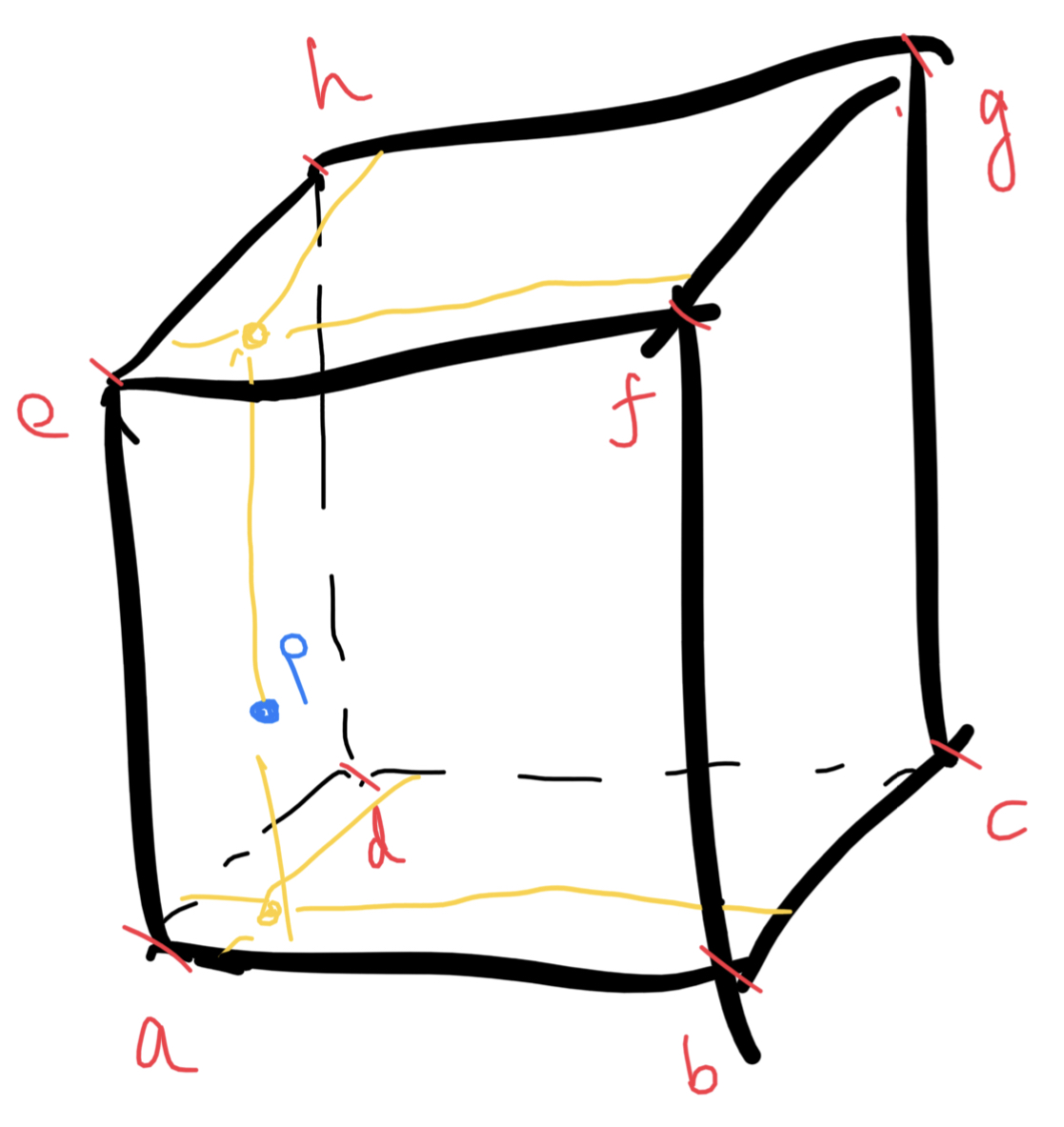
Given a sample point p, We do this via sampling the value noise values of the 8 vertices of the current sample cube cell, and linearly interpolate the values to obtain the result. So instead of bilinear interpolation in 2D noise functions, we now have trilinear interpolation:
The 3D value noise requires a 3D hash function:
float rand(vec3 p)
{
    return fract(sin(dot(p, vec3(12.345, 67.89, 412.12))) * 42123.45) * 2.0 - 1.0;
}
We have effectively implemented a 3D value noise function. But how do we really know we have implemented it correctly? Easy! We visualize it, using time as the third axis. We should be able to see the visualized noise changes smoothly over time:
Even though this is 3D, One problem you might’ve realized is that this is not very cloud-like. So what should we do to make it even more cloud-like?
fBm
Fractional Brownian motion, or fractal Brownian motion is, simply put, a “noise pass” in Computer Graphics. It can be applied to all kinds of noise algorithms. Inigo Quilez has an article on it; or, if you want a more intuitive understanding, and hands-on approach, you can try the Book of Shaders. It is also known as the “random walk process”, and here is an article which explains it more on the mathematic side.
Simply put, imagine we have a set of noise functions, which in our case is valueNoise1, valueNoise2, …, and for every point p, we do the following:
- Sample the noise value at point p: valueNoise1(p)
- Add its contribution to the final noise value weighted by w
- Cut w in half, or decrease/devolve it to whatever you wish: w = w/2
- Sample the second noise function at point p: valueNoise2(p)
- Add its weighted contribution
- Repeat until the w degenerates, or the number of octaves is reached
It’s not hard to see that the sample value changes with every octave. Violent at first, since w is big (persumably, initially \(w = \frac{1}{2}\); so the full weight,) then as the weight gets smaller and smaller, the sample value moves up and down, becomes bigger or smaller, but everytime the change becomes more and more insignificant, until finally the w degenerates. This will produce a non-smooth, jagged noise, but at the same time, since the value noise is smooth by nature, as we zoom in, self-similar patterns will emerge, much like the mandelbrot set.
This is, obviously, computationally expensive, and if we get the fBm noise value of point p, assuming there are 8 octaves, then the hash function needs to be sampled 64 times. But it is what we have, and we are going to just go with it. For now.
The other problem is we don’t really have 8 3D value noise functions. We can, and we have the option, but don’t you think that’s a little bit too much? A simple solution would be just to use the same noise function over and over again, but everytime we change the sample point p so that it lands in a new noise function area. Like this:
float fbm(vec3 p)
{
    vec3 q = p;
    int numOctaves = 8;
    float weight = 0.5;
    float ret = 0.0;

    // fbm
    for (int i = 0; i < numOctaves; i++)
    {
        ret += weight * valueNoise(q);
        q *= 2.0;
        weight *= 0.5;
    }
    return clamp(ret, 0.0, 1.0);
}
This is how the fbm result looks like if we visualize the normalized valueNoise result:
Feels very cloudy, does it not? But this feels like we are inside the cloud. A slight adjustment to the return statement is suffice if an illusion of us traveling above the cloud is needed:
return clamp(ret - p.y, 0.0, 1.0);
As sample point goes up, the fbm result becomes more and more sprase; and as sample point goes down, the cloud gets denser and denser, eventually clamping at 0 and 1. This is how it looks like:
Even though yes, it does look cloud-like, but so far we are only visualizing slices (with the slice index being time). The actual raymarched clouds are yet to be seen. So how do we raymarch volumetric things, exactly?
Volumetric Raymarching
Volumetric Raymarching is very similar to raymarching, except since we are marching over something that does not have a clear-defined shape, we have to assume we are hitting the volume every time. In practice, this can be optimized by placing a bounding box over it, but since this is just a tutorial, we are just going to assume we are always inside the volume.
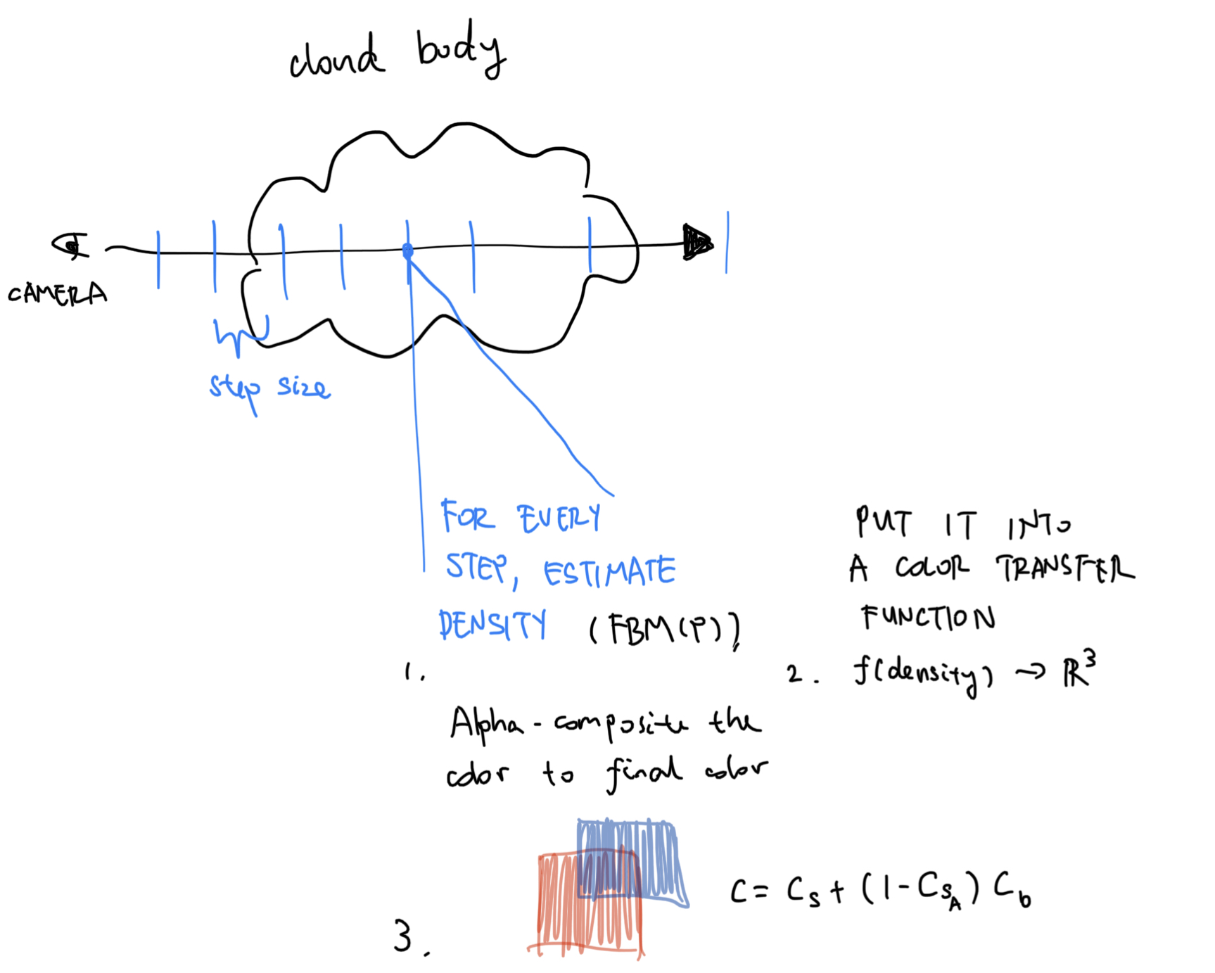
Since we are always hitting the cloud every step of the way, the usual raymarching step forward does not work here - the closest distance to object will always be 0. As a result, we will have to place our bets on fixed distance raymarching. Here’s a very general idea of what we are going to do:
And here’s the code for volumetric raymarching:
vec3 volumetricMarch(vec3 ro, vec3 rd)
{
    float depth = 0.0;
    vec4 color = vec4(0.0, 0.0, 0.0, 0.0);

    for (int i = 0; i < 150; i++)
    {
        // Standard raymarching procedure; #1
        vec3 p = ro + depth * rd;

        // Sample cloud density at point p; #2
        float density = fbm(p);

        // If density is unignorable...; #3
        if (density > 1e-3)
        {
            // We estimate the color with w.r.t. density; #4
            vec4 c = vec4(mix(vec3(1.0, 1.0, 1.0), vec3(0.0, 0.0, 0.0), density), density);
            c.a *= 0.4; // #5
            c.rgb *= c.a; // #6
            color += c * (1.0 - color.a); // #7
        }

        // March forward
        depth += max(0.05, 0.02 * depth); // #8
    }

    return clamp(color.rgb, 0.0, 1.0);
}
We can learn from #1 and #2 that this is just a standard raymarching procedure. #2 is akin to the map function; except we are not sampling for the signed distance field, but rather, a density field.
Since fbm is based on repetitive sampling of valueNoise, the result will range from \([-1, 1]\). If the result is more than 1e-3, which means the density becomes unignorable, and if that’s the case, we will need to take the density sampled into account for the final color.
#4 determines the cloud color at this particular spot - for demonstration purposes, the denser it is, the darker it gets. Then, in #6, we treat the density as alpha and dim the color contribution accordingly; and finally in #7, we composite the result to our final output color.
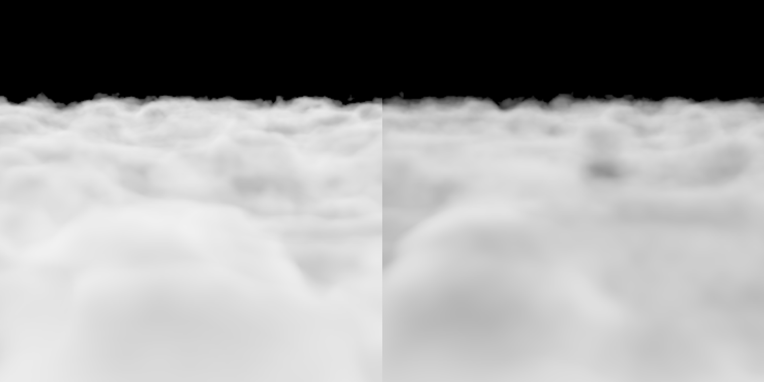
We can see from #7 that color.a can only go up - everytime a value equivalent to the cloud density at that spot is added. However, if we are sampling a high density cloud region, color.a might fill up too quickly, leaving the details behind unseen. To fix that we can weight the c.a with a fixed value, so that more cloud samples can contribute to the final color, giving us a smoother final render (right).
A big problem with fixed-step raymarching is the limited viewing distance. If we only march forward 0.05 meters everytime, 100 raymarching steps means a viewing distance of 5 meters, and that is way too short. When we move further and further away from the camera, the details should matter less and less, so we can try taking bigger steps when the distance is far enough, hence the max statement in #8.
And there we have it! Clouds in the sky. Here is a brief summary, a recipe, of raymarching clouds:
- Standard raymarching procedure.
- Sample the volume density at point p.
- The density could be used to determine cloud color at that particular point - this can be done by using a transfer function. In our case, the higher density the cloud is, the darker it becomes.
- We multiply the alpha channel of the color so the ray can penetrate deeper into the volume, and as a result, appear softer.
- The cloud color is composited to the final output color at that pixel, in a front-to-back order.
Here’s the code we have so far:
float rand(vec3 p)
{
    return fract(sin(dot(p, vec3(12.345, 67.89, 412.12))) * 42123.45) * 2.0 - 1.0;
}

float valueNoise(vec3 p)
{
    vec3 u = floor(p);
    vec3 v = fract(p);
    vec3 s = smoothstep(0.0, 1.0, v);

    float a = rand(u);
    float b = rand(u + vec3(1.0, 0.0, 0.0));
    float c = rand(u + vec3(0.0, 1.0, 0.0));
    float d = rand(u + vec3(1.0, 1.0, 0.0));
    float e = rand(u + vec3(0.0, 0.0, 1.0));
    float f = rand(u + vec3(1.0, 0.0, 1.0));
    float g = rand(u + vec3(0.0, 1.0, 1.0));
    float h = rand(u + vec3(1.0, 1.0, 1.0));

    return mix(mix(mix(a, b, s.x), mix(c, d, s.x), s.y),
               mix(mix(e, f, s.x), mix(g, h, s.x), s.y),
               s.z);
}

float fbm(vec3 p)
{
    vec3 q = p - vec3(0.1, 0.0, 0.0) * iTime;
    int numOctaves = 8;
    float weight = 0.5;
    float ret = 0.0;

    // fbm
    for (int i = 0; i < numOctaves; i++)
    {
        ret += weight * valueNoise(q);
        q *= 2.0;
        weight *= 0.5;
    }
    return clamp(ret - p.y, 0.0, 1.0);
}

vec3 volumetricMarch(vec3 ro, vec3 rd)
{
    float depth = 0.0;
    vec4 color = vec4(0.0, 0.0, 0.0, 0.0);

    for (int i = 0; i < 150; i++)
    {
        vec3 p = ro + depth * rd;
        float density = fbm(p);

        // If density is unignorable...
        if (density > 1e-3)
        {
            // We estimate the color with w.r.t. density
            vec4 c = vec4(mix(vec3(1.0, 1.0, 1.0), vec3(0.0, 0.0, 0.0), density), density);
            // Multiply it by a factor so that it becomes softer
            c.a *= 0.4;
            c.rgb *= c.a;
            color += c * (1.0 - color.a);
        }

        // March forward a fixed distance
        depth += max(0.05, 0.02 * depth);
    }

    return clamp(color.rgb, 0.0, 1.0);
}

void mainImage(out vec4 fragColor, in vec2 fragCoord)
{
    vec2 uv = (fragCoord.xy / iResolution.xy) * 2.0 - 1.0;
    vec3 ro = vec3(0.0, 1.0, iTime);
    vec3 front = normalize(vec3(0.0, -0.3, 1.0));
    vec3 right = normalize(cross(front, vec3(0.0, 1.0, 0.0)));
    vec3 up = normalize(cross(right, front));
    mat3 lookAt = mat3(right, up, front);
    vec3 rd = lookAt * normalize(vec3(uv, 1.0));
    vec3 cloudColor = volumetricMarch(ro, rd);

    // Gamma correction
    cloudColor = pow(cloudColor, vec3(0.4545));

    fragColor = vec4(
        cloudColor,
        1.0);
}
Further Readings & Improvements
The cloud shader can, of course, be vastly improved in both rendering quality and optimizations. The very first thing that comes to mind is the method above is still not cloud-like enough. My fBm cloud method is too brute-forced; compared to how the fBm should look like originally, only the boundaries exhibit cloud-like behavior. So that could be vastly improved.
Another noticable artifact is far away clouds, which should stay hidden due to strong aliasing. An easy fix would be hide it with fog, so the further away it is, the more blended-in it is with the background. Or, like the Cloud Shader by Inigo Quilez, use an exponential fog equation to achieve better effect.
Another one is speed. It’s too slow for everything to be calculated in the shader. A 3D noise texture could be used for faster noise sampling. A simple textureLod command is way faster than 8 value noises calls and a trilinear interpolation.
And then there’s the problem of the cloud being unshaded. But that’s up to you! Some background and a custom-made color transfer function later, it can look pretty good:
Some additional clouds & volume rendering related techniques & tutorials:
- Volume Rendering for Developers: Foundations on Scratchapixel.
- NVIDIA’s GPU Gems Chapter 39: Volume Rendering. Note, this only covers texture-based volume rendering.
- Volume Rendering blog post by Matias Lavik, also known as @sigsegv@floss.social.
You can check out my shaded cloud shader on Shadertoy. Or, you can view it below.
Comments