This is a blog post from the past. Originally written at 2021-12-03.

In case you didn’t know, I am learning those stuffs from CMU 15-462. The title image is (kinda) an assignment from this video in particular. Prof. Keenan Crane is awesome!

What are linear transformations?

Linear transformations are also called linear maps. Not strictly speaking, linear transformations must satisfy:

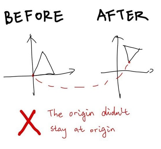
1. After the transformation, the origin stays at origin
2. Additivity: Conforms \(f(x+y) = f(x) + f(y)\)
3. Homogeneity: \(c f(x) = f(c x)\)

Not strictly speaking (again), after a linear transformation, straight lines should remain straight lines.

What are the basic type of linear transformations?

Scaling

It’s very easy to scale something along an axis: you just multiply a number with a constant value \(c\): \(c\begin{bmatrix}x_0 \cr x_1 \end{bmatrix}\).

It’s very easy to transform this operation into a matrix multiplication, because what we just did above is equivalent to

And if we want nonuniform transformations along the axis, we just don’t make the first matrix all \(c\)s. We can maybe have a \(diag(1, 5, 8)\) to make the y axis 5 times longer and z axis 8 times longer, while the x axis remains unchanged. That’s pretty simple.

Rotation

Imagine there’s a 2D plane. Now imagine the two basis vectors: \(e_0 := \begin{bmatrix}1 \cr 0\end{bmatrix}\) and \(e_1 := \begin{bmatrix}0 \cr 1\end{bmatrix}\). In order to rotate \(e_0\) for \(\theta\) degrees, you will find that it is equivalent to function \(f(\theta) = \begin{bmatrix}cos(\theta) \cr sin(\theta)\end{bmatrix}\) evaluated at \(\theta = \frac{\pi}{2}\). Its norm also remains 1 because \(sin^2(x) + cos^2(x) = 1\). So that’s pretty cool.

Now, when the same thing needs to be done for \(e_1\), it’s pretty clear that \(e_1\) is just \(e_0\) with a headstart rotation of 90 degrees, so the rotation of \(e_1\) is simply \(f(\theta) = \begin{bmatrix}cos(\theta + \frac{\pi}{2}) \cr sin(\theta + \frac{\pi}{2})\end{bmatrix} = \begin{bmatrix}-sin(\theta) \cr cos(\theta)\end{bmatrix}\).

Now, \(e_0\) is just \(1 \times e_0 + 0 \times e_1\). The same goes for \(e_1\). Since they form the basis vectors, every vectors in the 2D plane can be decomposed into a linear combination of \(e_0\) and \(e_1\), for example:

This could be written, in the matrix multiplication form, as

… And it’s pretty clear where this is going. Rotating for \(\theta\) degrees really just means defining two new basis vectors above, \(\begin{bmatrix}cos(\theta) \cr sin(\theta)\end{bmatrix}\) and \(\begin{bmatrix}-sin(\theta) \cr cos(\theta)\end{bmatrix}\). Combining them together, and plugging in the basis-vector-matrix thingy above, we get

That’s it!

What About 3D Then?

We can achieve 3D rotation by fixing the third coordinate. For example,

This fixes the z axis and rotates the xy plane. Or, as we call it in 3D, “rotate along the z axis”. The same can be done for x axis and y axis:

The transpose of the rotation matrix \(R^T\) is the inverse of \(R\), meaning \(R^TR = I\). You can try multiplying them if you don’t trust this conclusion.

Non-uniform Scaling

The two operations above, rotation and scaling, allows for nonuniform scaling. If there’s this cube, but we don’t want to scale it along the x axis, but some arbitrary vector \(v\), we can rotate it there first, and then scale, and then rotate back.

The result of a composited nonuniform scaling matrix will be a symmetric matrix (and all symmetric matrices will be nonuniform scaling matrices because spectral theorem says so).

Shearing

Shearing is the process of displacing the point \(x\) in the direction \(u\) based on its alignment with vector \(v\).

Shearing a vector \(x\) based on \(u\) and \(v\) looks like this:

How to understand shearing? If we have two basis vectors \(i\) and \(j\), then after shearing, \(\hat{i} = i + \langle v, i \rangle u\), \(\hat{j} = j + \langle v, j \rangle u\). And for whatever point in the original space \(p\), the new position will be \(\hat{p} = \begin{bmatrix}\hat{i} & \hat{j}\end{bmatrix} p\). The 2D shearing matrix can thus be defined as:

3D shearing is just 2D shearing with extra steps.

All those three are linear transformations. Their origin doesn’t change, they have homogeneity and additivity, and all of them have a matrix representation. This means that they can be conveniently composited into a single matrix, and it can then be used to be applied to a point or vector.

But there is still one more. the translation. There are no way to translate points in space! Why?

Translation

That’s because translation is not linear. It’s pretty simple - after a translation, the origin probably isn’t going to stay the same. Translation is an affine transformation. However, the introduction of homogeneous coordinate can (easily?) fix that.

Homogeneous Coordinate

Imagine a 2D plane. Now imagine that we describe every point in the 2D plane like this:

The points didn’t really change, we just kinda put them into a slice of the 3D space. It’s like we are viewing a thin slice of cake now.

Does it make any sense to you? No? Well, you are going to see why does this make sense pretty soon.

3D Shearing is 2D Translation

Suppose we are doing a 3D shearing along the \(v = \begin{bmatrix}0 \cr 0 \cr 1\end{bmatrix}\) axis with the offset \(u = \begin{bmatrix}-1 \cr 0 \cr 0\end{bmatrix}\). What happens? We can construct a shearing matrix like so and plug in random numbers to see what happens:

Now, if you are a curious boy/girl and plug in the homogeneous coordinate above, you will notice something strange:>

If we ignore the \(z\) axis, we can notice that \(p\) has shifted by \(\begin{bmatrix}-1 \cr 0\end{bmatrix}\). We have achieved translation, and it’s a linear transformation too! The only small price to pay is that we will have to add an extra dimension.

It doesn’t matter in computer graphics anyway, since this is not the only usage of homogeneous coordinate, as it is also used to perform perspective divides. So it’s a win-win for us all - a translation that is also a linear transformation, and a super easy way to make perspective camera. Awesome!

With homogeneous coordinate in our hand, defining a translation matrix is easy:

All other linear transformations, simply need to add \(\begin{bmatrix}0 \cr 0 \cr 0 \cr 1\end{bmatrix}\) when introduced to the homogeneous space.

Scene Graph

With all those matrices (or rather, the knowledge of how basis vectors should transform) in hand, we can describe rotation, translation, and scaling, and probably more. All other weird funky affine transformations can be done by compositing all the matrices above.

Note that matrix multiplication is non-commutative, so you can’t swap the orders around. It makes sense, because translate \(\rightarrow\) rotate is different from rotate \(\rightarrow\) translate.

It is then possible to describe a scene, such as flowers on a table, so that when the table rotate, the flower rotates with the table (otherwise it’s gonna be weird.) How can we achieve that? With composite transformations, of course - the flower has its own pose & transformations, and is meanwhile under the table’s influence, too. This can be achieved by applying the transformation matrices to the flower first, then apply the transformation of the table to the flower as well:

This can be easily done by a scene graph:

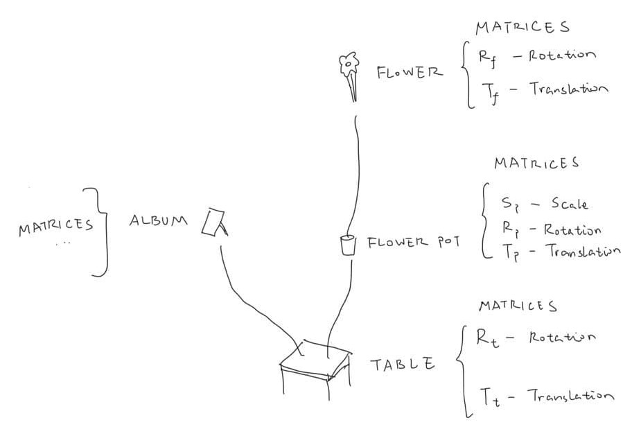
How does this happen in actual code? It’s just a tree data structure with table as the root node. The transformations of objects are pre-composited, so for example the table data structure will be:

Table {
    Children = { Flower pot, Album }
    Transformation = T * R
}

When we are actually going to render a frame, we will traverse this tree known as scene graph in a depth-first search order. So we will render the table first, after applying the table’s transformation - then we will actually put the table’s transformation matrix into a stack.

Now we will go to the table’s children. It’s the flower pot, so we apply the flower pot’s transformation to all flower pot’s points. Then, we apply all transformations in the current stack - in this case the table’s transformation. In this way, the flower pot rotates and translates with the table. After that’s done, we also put the flower pot’s transformation matrix into the stack.

The same goes for the flower. Now the flower will be transformed by the flower pot and the table. You can probably see where this is going - after the traversal finishes, we can revert the stack to its previous state by popping it.

Skeletal Animation

Using scene graph is a very useful way to describe skeletal animation. The head is affected by the body, the fingers are affected by the hands, etc. Using all the knowledge we have now, we can actually make a skeletal animation of a boxy dude waving.

Comments

A valid, non-empty username is required.

Comment