Grass is a beautiful thing. I can still remember when I was very small, and I was just getting a brand new Sony Ericsson phone - was it the Xperia Duo? Anyway, among the things I discovered, the most memorable one is the live wallpaper Grass. A few grass blades swaying gently under a blue sky, and the sky & lighting changes throughout the day. It was a big aesthetic update from my last phone, which was Nokia 5300, and my mind was blown. I fell in love with rendered grass ever since.

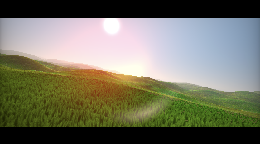
So, let’s render some grass! The shader we’ll be referencing is Rolling Hills by Dave Hoskins. First, please appreciate its stunning beauty:

Worley Noise

The first thing we need to do is generate a grass-like pattern, so that we actually have things to raymarch into. A 3D Worley noise would suffice.

In case you don’t know how Worley Noise works, it’s a noise algorithm which very much looks like a Voronoi diagram. It’s also called Voronoi noise, or cellular noise, because of its cell-like nature; there is a detailed explanation & implementation in the Book of Shaders. Here’s a concise explanation:

1. Divide the shading area into a series of cells. A simple floor operation is enough.
2. Generate a random point for each cell. This can be done via the hash function.
3. For the current shading point, find & record its closest distance (and cell) to all the random point in neighboring cells.
4. Shade accordingly.

vec2 voronoi(vec2 uv)
{
    // Use time to warp the space
    vec2 f = fract(uv);
    vec2 u = floor(uv);
    
    float closest = 100.0;
    float id = 0.0;
    for (int y = -1; y <= 1; y++)
    {
        for (int x = -1; x <= 1; x++)
        {
            vec2 d = vec2(float(x), float(y));
            vec2 nu = u + d;
            vec2 p = hash22(nu);
            float dist = distance(f, p + d);
            if (dist < closest)
            {
                closest = dist;
                id = hash(nu);
            }
        }
    }
    return vec2(max(0.0, 1.0 - closest), id);
}

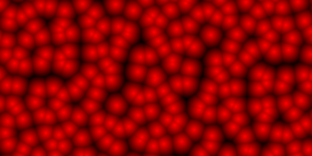
Instead of using the closest value directly, we invert it so that the center becomes very large, while the boundaries become small. In this way, we can describe a the density of a horizontal slice of grass - and voronoi(uv) == 0 indicates its boundary.

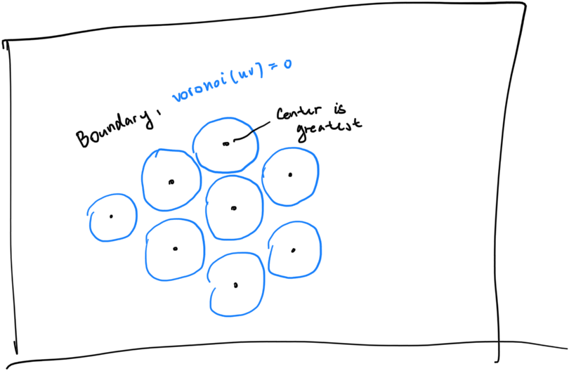
Here’s a visualization.

3D Worley Noise

And now, it’s time to elevate it to the third dimension. The Worley noise above describes the grass at \(y = 0\). As the sampling y goes up, the grass blades should become thinner and thinner, eventually converging at the top.

vec3 voronoi_3d(vec3 p)
{
    float grassHeight = 1.0;
    
    vec2 uv = p.xz * 3.0;
    float id = voronoi(uv).y;

    vec2 vor = voronoi(uv);
    float boundary = mix(0.0, 1.0, max(p.y / grassHeight, 0.0));
    
    return vec3(boundary - vor.x, vor.x - boundary, vor.y);
}

As sampling height goes up, boundary becomes larger and larger and eventually reaches 1, which is the maximum possible return value of our voronoi function above. Now when the sampling height is zero, Worley noise’s return value is simply inverted; this turns the return density into a horizontal SDF. The second return value denotes the density modified with height, and the third return value denotes the hashed Worley cell ID. A visualization of what happens as sampling y goes up is presented below.

Volumetric Raymarching

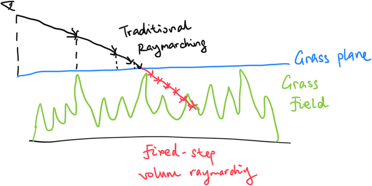
And now with the grass kinda SDF in hand, it’s time for us to render it. Since the grass kinda SDF is really just the SDF of a horizontal slice, we don’t know its exact 3D SDF, and as a result, can’t really use traditional raymarching method. We can however turn this into an volumetric raymarching endeavour - the ray marches forward in fixed steps and we blend the result.

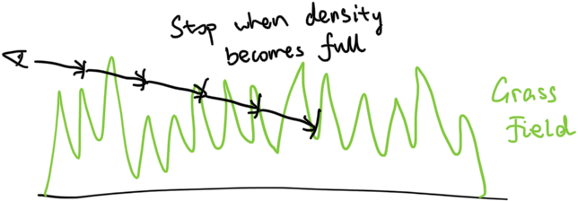
But fixed-step volume raymarching is very expensive. To optimize it, we can actually perform traditional raymarch first - up until the ray hits the tallest grass surface. Then we begin volume raymarching.

Since our grassHeight is defined at 1.0, our floor SDF ground can be easily defined:

float ground(vec3 p, out vec3 mat)
{
    mat = vec3(0.2, 0.4, 0.1); 
    return p.y - 1.0;
}

The rest is just normal raymarching procedure, up until the ray hits the ground and we need to shade it. Then, we perform volumetric raymarching into the grass field defined above. Here’s a general idea:

vec4 grassBlades(vec3 ro, vec3 rd, float t)
{
    vec3 grassColor = vec3(0.0);
    vec4 color = vec4(0.0, 0.0, 0.0, 0.0);
    
    for (int i = 0; i < 100; i++)
    {
        vec3 p = ro + t * rd + base;
        
        vec3 grass = voronoi_3d(p);
        t += max(0.001, t * 0.04);
        
        // If we are outside the grass field...
        if (grass.x > 0.0)
        {
            continue;
        }

        float den = clamp(min(grass.y, 1.0 - color.a), 0.0, 1.0);
        //
        // The denser it is, the darker it is
        //
        vec3 bladeColor = mix(vec3(0.0, 0.0, 0.0), vec3(1.0, 1.0, 1.0), den);

        color.rgb = color.rgb + bladeColor * den;
        color.a += den;
        if (color.a > 0.99)
        {
            break;
        }
    }

    return color;
}

And that’s the core idea! However, if you are following what we’ve been doing so far, the grass you’ve gotten should not be satisfactory. However fret not! Since we already have the basic idea, by adjusting a lot of parameters and turning a lot of knobs, we can always achieve our desired result. Here are a few recommendations:

1. Raymarching step size and total # of raymarching steps: tuning the step size down and number of steps up can increase the overall crispiness and viewing distance of the grass.
2. Base volumetric raymarching coordinate offset: by having a simple negative y offset for the volumetric raymarching sampling coordinate, we can start raymarching inside the grass field, which is very convenient and saves a lot of time. This is very useful. Refer to Fig. 1 and Fig. 2 for comparisons.
3. Grass color: adjusting the grass color can achieve different aesthetic effects. You can make real grass or cartoon grass.
4. Worley noise 3D sampling coordinate: by applying a small height-based rotation to the grass field function, we can emulate wind. Refer to the final video to see it work in action.
5. … and a lot more!

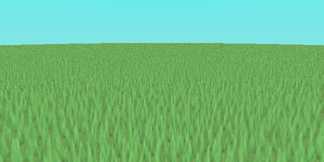
Fig. 1 without the simple offset. Notice the obvious banding in the distance. The grass is also way more blurry.

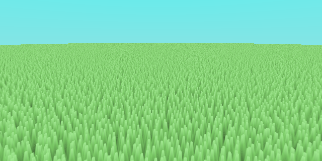
Fig. 2 with the simple offset.

The final result has a big downside - I had not implemented a terrain system. So yes, even though there are grass, they have to be situated on a perfectly flat surface. I have tried adding Perlin noise to that, but alas, it did not work in my favor, and I am running short on time. Nonetheless, here’s my final shader: a (cartoonish) grass field gently swaying under a blue sky. It is also available on Shadertoy. Go check it out!

Comments

A valid, non-empty username is required.

Comment