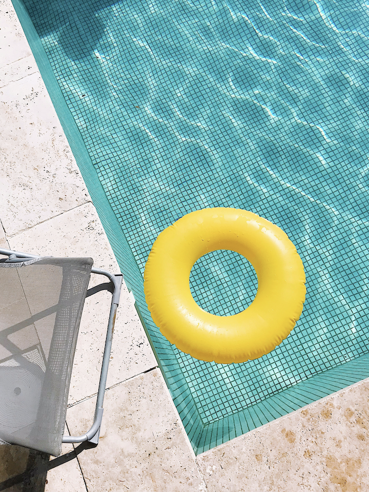
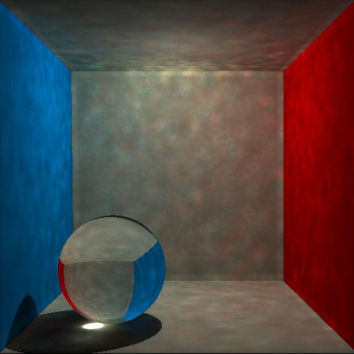
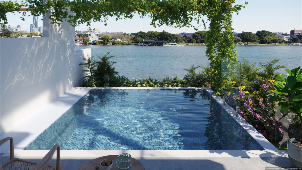
Photon Mapping is a rendering algorithm developed by Henrik Wann Jensen to specifically tackle the problem of rendering caustics. Caustics are beautiful optical phenomena created by light rays passing refractive surfaces, like water or glass, and concentrated onto the same spot, creating a bright patch of light. Like this one (notice the bottom of the pool):

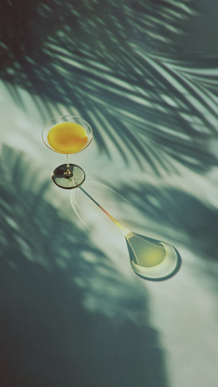
Or, take a look at the shadow of this wine glass:

Extraordinary, aren’t they? Too bad they are a PITA to trace and render using conventional raytracing techniques. Let’s take a look at why, and how Jensen solves the problem.

Why Are Caustics Hard?

To understand why caustics are hard, we must understand how raytracing works. Let’s first take a step back, and discuss how we see things as they are. Scratchapixel provides excellent explanation for this. But in a nutshell, the light sources, lamps, sun, etc., are constantly shooting out an incomprehensible amount of photons at all times. These photons bounces around wildly, and some of them, after many bounces, lands in our retina.

In reality though, rendering this way is far too expensive. We have wasted tons of calculations on what we eventually can’t see (since most light rays won’t end up in the camera anyway), and those are just wasted calculations. Luckily, according to the reversibility principle, if light can travel from path A to B, it can travel back from B to A. This is why we trace rays from the camera instead. This forms the foundation of most path tracing algorithms.

Although path tracing is certainly better than forward raytracing, the noise problem remains. Most of the rays shooting out from the camera won’t reach the light. And as the light gets smaller, it becomes less possible for the rays to hit said light, making the final image nosier and nosier. Image stolen from Chaos.

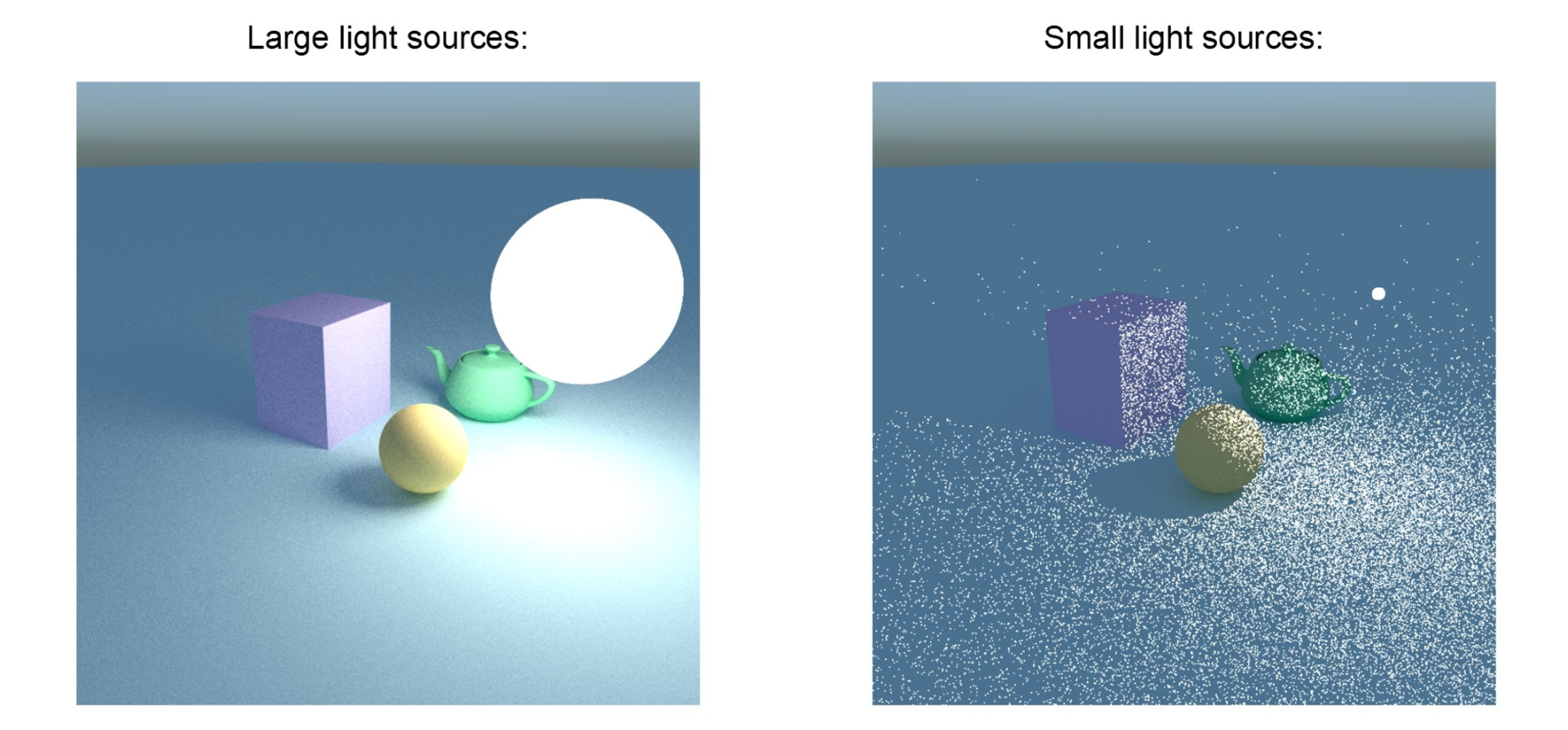
No one wants noisy images, so the graphics folks came up with a solution: importance sampling. Now when we are reflecting light rays, we purposefully direct it towards the light source, and weight it accordingly. Now there are less wasted calculations, and the final image is less noisy. Horray! Everyone wins.

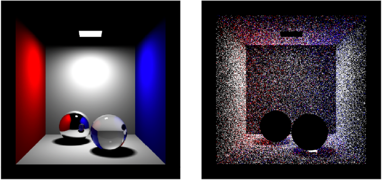
However, doing so creates a new problem. When we are tracing lights through refractive materials, what will original lead us to the light might now miss completely due to the light ray being refracted when passing through the object. This leads to, again, wasted calculations, and noisy final image. So how can we solve it?

Photon Mapping

Enter photon mapping. Proposed by Jensen in 1996, the original paper is available online here. Jensen proposes a two-pass method to construct a photon map. In the first pass, photons are emitted from the photon map, in the number of tens of thousands. Everytime a photon interacts with a diffuse surface, we deposit the interaction information into a photon map. The photon map will store the following:

1. Interaction position \(p\): where the interaction happened.
2. Incoming ray direction \(\omega_i\), the direction the photon was coming from.
3. Photon power \(dE\): Since photons represents incoming flux, one single photon is representative of differential flux.

After storing it into a diffuse surface, now we determine if the surface should absorb the photon, or reflect the photon. Russian roulette is used to determine if we should stop tracing. An example is shown here by Jensen:

// Surface reflectance: R = 0.5 
// Incoming photon: Φp = 2 W

r = random();
if(r < 0.5)
    reflect photon with power 2 W
else
    photon is absorbed

There are actually two photon maps to construct, one called “Global Photon Map” and the other “Caustics Photon Map”. The way caustics photon maps are constructed is just slightly different than global photon maps: photons are emitted from the light source but now they aim directly at refractive objects. Think about importance sampling, but this time we are not aiming at lights, but rather water, or glass. When a photon is found conforming to the LS+D (light source - specular object - diffuse surface) path, we add that to the caustics photon map as well.

Constructed photon maps are stored in the format of a K-d tree (usually in the form of an octree) so that they can be accessed quickly. Here’s the approximate result of a constructed photon map:

Rendering

After contructing the photon map, now it’s time for us to render. The first step of rendering using a photon map is basically the same as path tracing. Rays are shot out from the camera, and then for every ray, we check if they had hit a surface. After a ray-surface interaction has been found though, things begin to change. Let’s take a look back at the Rendering Equation:

The Rendering Equation states that the radiance of a point towards direction \(\omega_o\) is the combination of its irradiance towards \(\omega_o\) and the indirect lighting coming from a hemisphere. But since a photon map is already in place for us, we can exploit that and split the incoming radiance into four parts: direct illumination, specular reflection, caustics, and soft indirect illumination:

Where \(L_r\) is

And

\(L_{i, d}\) represents direct illumination, \(L_{i, l}\) represents light sources coming from a specular reflection (caustics), and \(L_{i, c}\) represents indirect soft illumination.

Direct Illumination and Specular Reflection

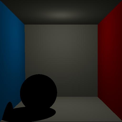
The first and second part of the incoming radiance contribution is calculated as if we are doing direct illumination in a regular path tracer. When a ray interacts with a surface, we evaluate its direct illumination by importance sampling towards the light source. Or if the surface is specular, then we trace the sample ray by reflecting it based on the surface normal. Nothing else is added. Here’s how a direct-illuminated scene looks like (taken from Brian Matejek’s Photon Tracing course):

Indirect Illumination

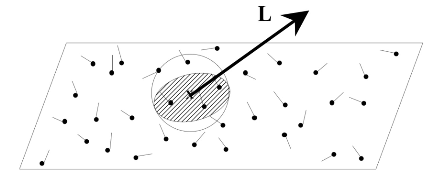
Indirect illumination (the 4th term) is light arrived after many bounces. Normally speaking, this means shooting out a ray towards a random direction. The more rays we shoot, the more correct the indirect illumination is. However, recall that a photon mapping is already in place, which is photons traced from the light source. All we need to do is to gather our k-nearest photon samples, integrate them together, and we’re as good as doing a Monte-Carlo integration.

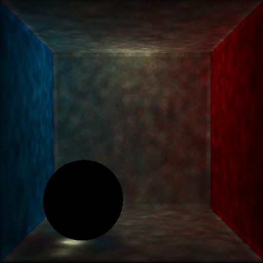
Here’s the indirectly illuminated scene, integrated using the global photon map:

Caustics

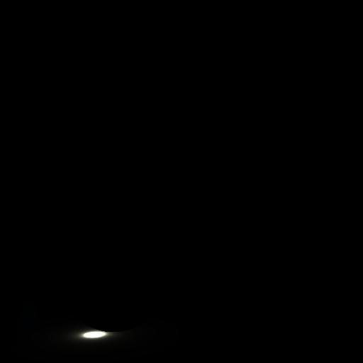
Caustics (the 3rd term) evaluates the effect the photon mapping paper is trying to achieve: caustics. It’s pretty much the same with indirect illumination, only this time contribution is calculated via the caustics photon map:

The four terms are combined together to produce a final colored image:

Conclusion

In conclusion, photon mapping achieves the caustics effect by using photon maps, which are k-d trees, which stores light path information traced from the light sources in the scene. These pieces of information are split into two photon maps, one for indirect lighting (global photon map), and one for caustics (caustics photon map).

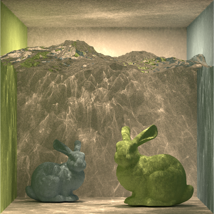
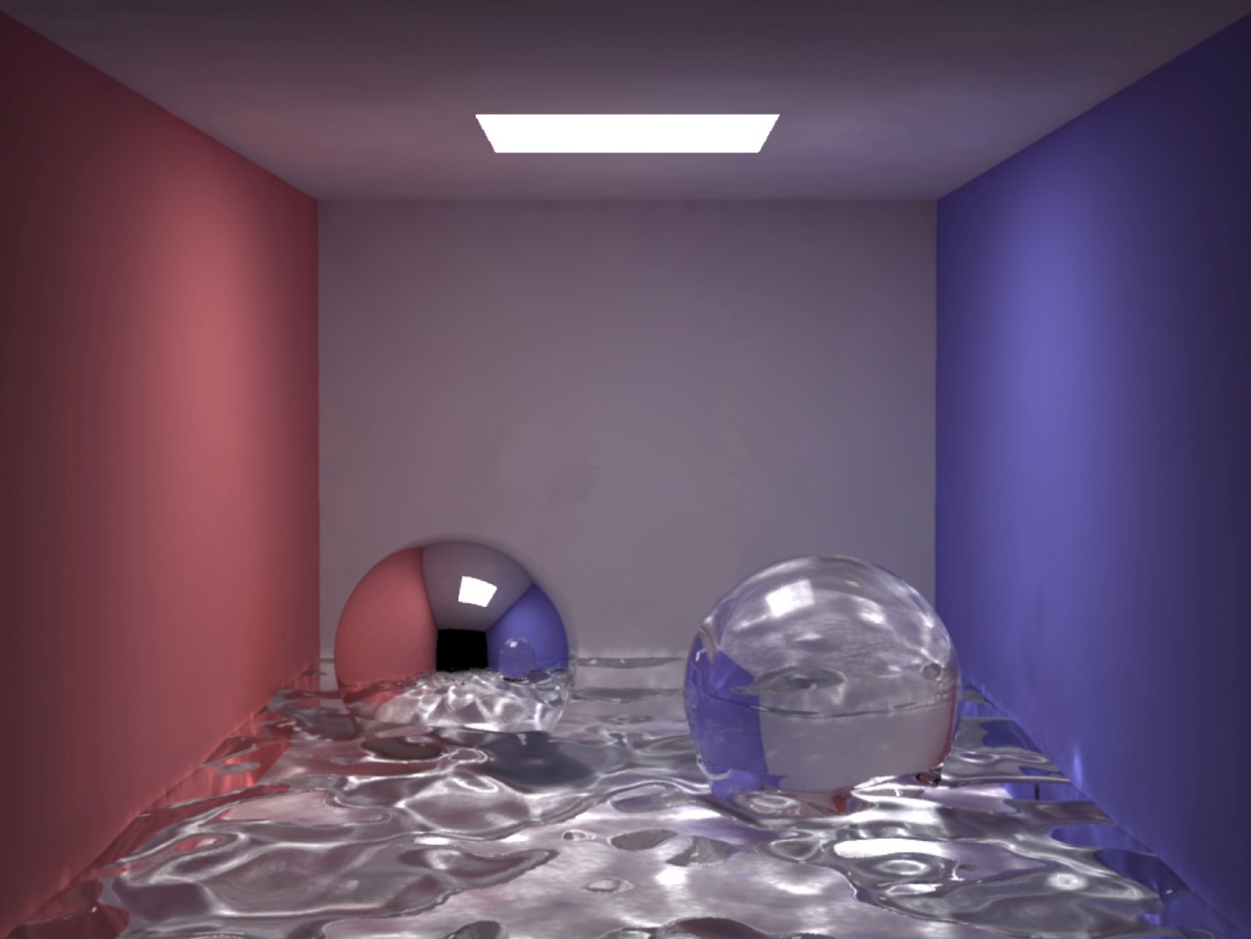
The rendering procedure behaves pretty much like a standard path tracer. Except when a ray-surface intersection is found, we don’t shoot out one direct light sample ray and one indirect light sample ray; rather, we shoot out a direct light sample ray, and calculate caustics and indirect lighting by gathering nearby photons. And that’s pretty much it! Now some real images, to show the full power of what photon mapping is capable of. And I will see you next time.

References

• Henrik Wann Jensen’s Global Illumination Using Photon Maps
• Photon Mapping writeup by Zack Waters
• Radiometry @ Cornell
• What are Caustics and How to Render Them the Right Way | Chaos Group
• Photon Mapping course at UC Davis
• Photon Mapping Made Easy
• Photon Mapping | Wikipedia
• Realistic Image Synthesis Using Photon Mapping
• Russian Roulette in Photon Mapping
• Photon Tracing

Comments

A valid, non-empty username is required.

Comment