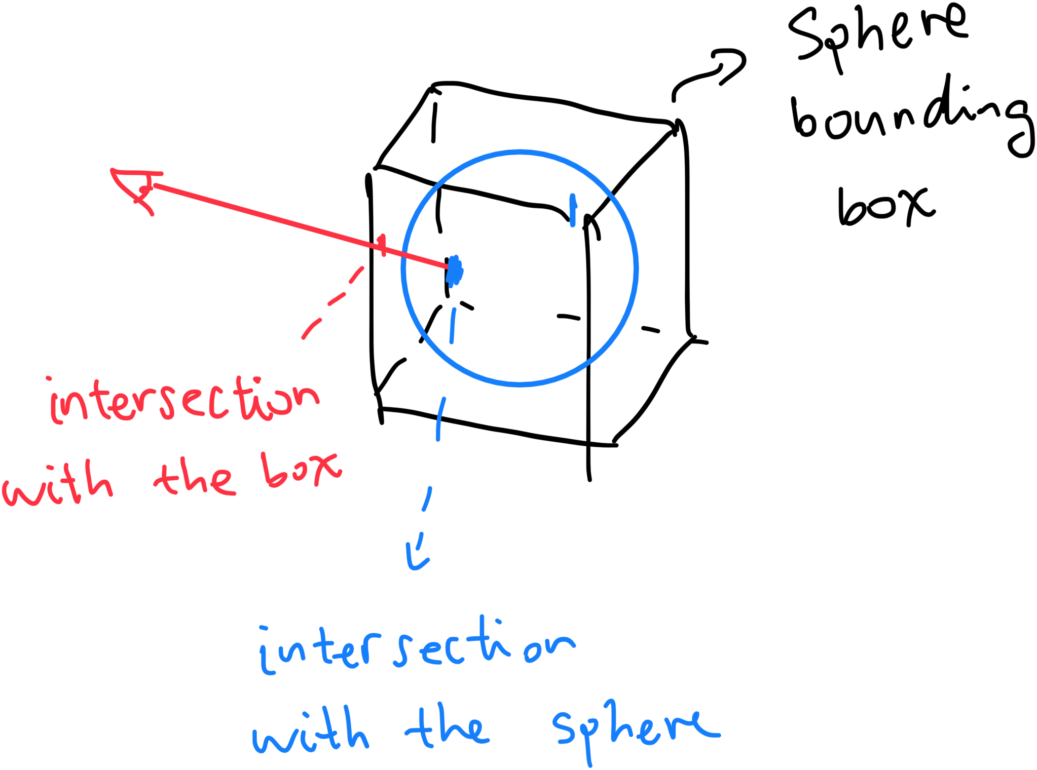
Have you ever wondered about how to render a perfect sphere in the OpenGL pipeline? “But we can only render points, lines, triangles and whatnot!” I heard you say, “so how?!” Well, screen-space raytracing, of course! We first render a box, then check if the camera intersects with the sphere inside the box. If it doesn’t, we discard it. Here’s how:

But now here comes the real problem: how is this “screen-space raytracing” done? Well, let’s take a look!

Ray-Sphere Intersection

As we are, in actuality, rendering a bounding box of the sphere, we have the world position of the pixel we are rendering in during the fragment processing pass. However, that world position is not the world position of our sphere. Rather, it is the world position of the bounding box, which almost always lies outside of the sphere, unless it’s the 6 tangent points. Nevertheless, we still need to calculate that first in the vertex shader:

#version 430 core

layout (location = 0) in vec3 aPos;

uniform mat4 model;
uniform mat4 view;
uniform mat4 perspective;

out vec3 worldPos;

void main() {
    vec4 wPos = model * vec4(aPos, 1.0);
    worldPos = vec3(wPos);
    gl_Position = perspective * view * wPos;
}

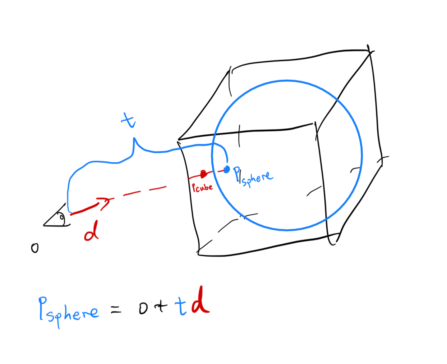
To recover the real world position of the shading fragment of our sphere, we need a ray-sphere intersection check. Luckily, we know the ray direction: since the box intersection point \(p_\text{box}\), sphere intersection point \(p_\text{sphere}\), and camera position \(o\) are colienar, we can deduce that ray direction

Let’s assume the sphere has a radius of 1. Assuming the ray does hit the sphere, the intersection point \(p_\text{sphere}\), which is on the sphere, its distance to the sphere center must equal to its radius (1).

So now we have

If we can solve for \(t\), we can know exactly where the sphere shading point is located. So let’s expand the above equation by raising both sides to the power of 2. And if you recall, the length of a vector is the square root of the dot product of the vector with itself. So:

Let’s represent \(o - c\) as \(u\). It represents camera’s relative position to the center of the sphere, i.e. Camera’s sphere-local coordinate. By throwing the 1.0 to the left side as well, the above equation can be rewritten as:

And now we further expand those dot operators and isolate \(t\):

Waaait a minute… Something is looking kind of fishy. We can bust out the quadratic equation solution formula!

Discriminant \(\Delta\) can be calculated using \(b^2 - 4 a c\). And if it is less than 0? That means the ray has no intersection with the sphere. This is definitely a thing:

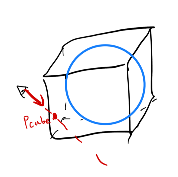
When this happens, we just discard the current fragment. No extra steps needed. And now, with the discriminant at hand, now the only thing left for us to do is to actually solve \(t\).

We will take the \(t\) with the smallest value, since the ray intersects the closer point (to us) first, not the further one. Now \(p_\text{sphere}\) can be properly recovered by using

#version 430 core

in vec3 worldPos;
out vec4 color;

uniform vec3 camPos;
uniform vec3 sphereCenter;

vec3 sphereIntersect(vec3 c, vec3 ro, vec3 p) {
    vec3 rd = vec3(normalize(p - ro));
    vec3 u = vec3(ro - c); // ro relative to c

    float a = dot(rd, rd);
    float b = 2.0 * dot(u, rd);
    float cc = dot(u, u) - 1.0;

    float discriminant = b * b - 4 * a * cc;

    // no intersection
    if (discriminant < 0.0) {
        return vec3(0.0);
    }

    float t1 = (-b + sqrt(discriminant)) / (2.0 * a);
    float t2 = (-b - sqrt(discriminant)) / (2.0 * a);
    float t = min(t1, t2);
    vec3 intersection = ro + vec3(t * rd);

    return intersection;
}

void main() {
    vec3 sp = sphereIntersect(sphereCenter, camPos, worldPos);
    if (sp == vec3(0.0)) {
        discard;
    }
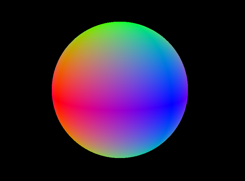
    color = vec4(abs(sp), 1.0);
}

The code should provide a perfect sphere. And it stays a sphere, even when you are very, very close to it.

Normal Calculation

You will find the above shaded result looks suspiciously like the normals of the sphere. Though we are shading the coordinates, it feels very normal-ly. And it is! Remember that we are shading a unit sphere, and the sphere I presented above is located at the dead center of the world, making the shading points equals to their normals. And even if the sphere is not located at the center, the normal is still simple enough to obtain. Just negative offset the \(p_\text{sphere}\) by the sphere center, and BAM! That’s our normal.

vec3 localIntersection = intersection - c;
normal = localIntersection;

Ellipsoid

Since we have already taken care of screen-space sphere raytracing, ellipsoid is basically free - with a few extra steps. Since we can treat ellipsoids like transformed spheres, we can assign two extra properties for our sphere:

1. The scaling of the ellipsoid \(s\).
2. The rotation of the ellipsoid \(R\);

During our tracing, we require that a sphere is first scaled, then rotated. If we rotate first, then the rotation will be meaningless - as spheres are rotation-invariant.

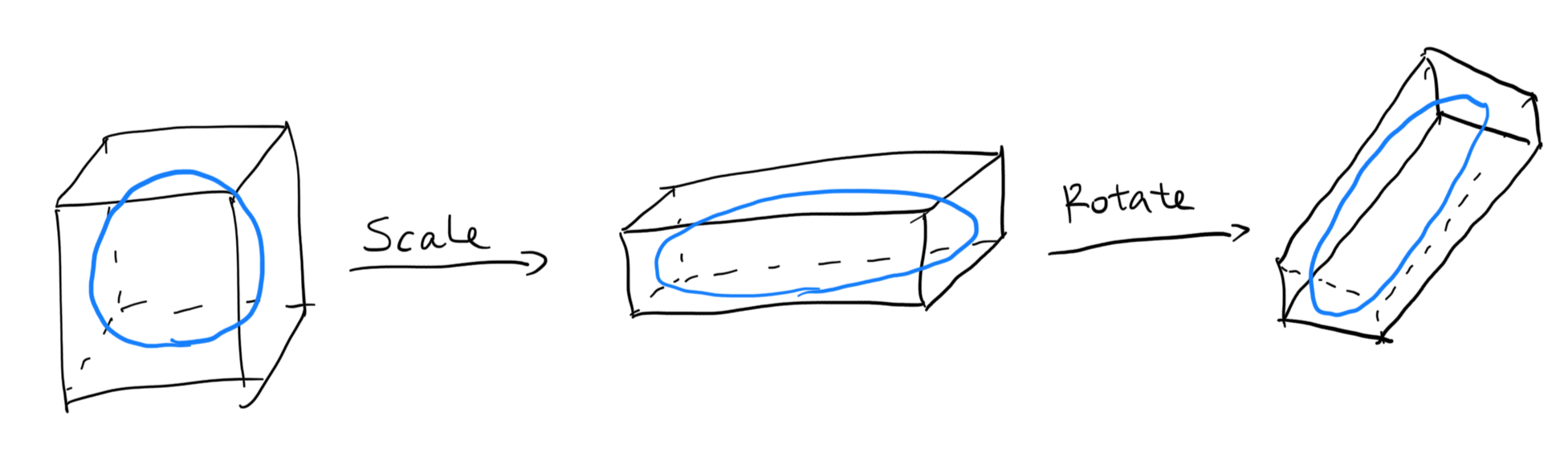
The scaling is not required to be uniform. As in, the scaling vector is not required to be equal on all axes. So now that we have these two vectors \(s\) and \(R\), how do we trace out the transformed sphere? Let’s go over scaling and rotation one by one.

Ellipsoid Scaling

To scale the inner ellipsoid, we need to first scale the outer bounding box, as the bounding box must contain the whole thing.

void Ellipsoid::compositeTransformations()
{
    // Composite transformations in the reverse order:
    // translate <- scale
    _model = glm::mat4(1.0f);
    _model = glm::translate(_model, _center);
    _model = glm::scale(_model, _scale);
}

Now that that’s out of the way, recall the sphere raytracing code above:

// We added a new "normal" output parameter
vec3 sphereIntersect(vec3 c, vec3 ro, vec3 p, out vec3 normal) {
    vec3 rd = vec3(normalize(p - ro));
    vec3 u = vec3(ro - c); // ro relative to c

    // ...

    vec3 intersection = ro + vec3(t * rd);
    vec3 localIntersection = intersection - c;
    normal = localIntersection;

    return intersection;
}

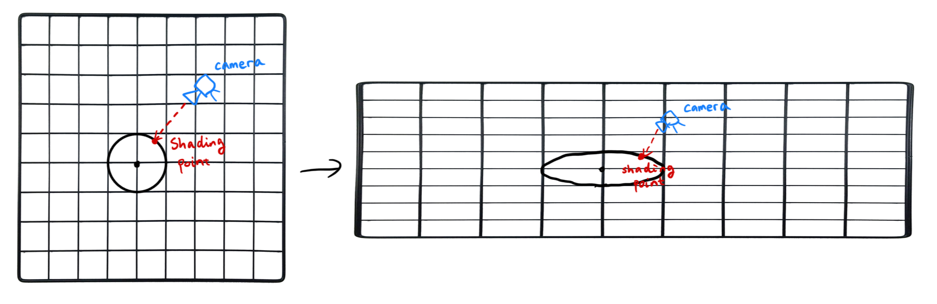
You might’ve noticed that the whole tracing procedure is done in local space. u is the relative camera origin to the sphere center, and rd is the incoming ray direction. This means not much modification is needed to achieve nonuniform sphere scaling: in lieu of transforming the sphere itself, we can reverse-transform the camera to the local space based on the sphere transforming parameters.

In other words, if the ellipsoid is scaled to get bigger, the relative camera position should be closer to the sphere, as it takes less spheres to get to the camera (because the unit of length in the local space grows). Perhaps an illustration is better.

To account for this, we apply the inverse scaling to both the ray direction rd and relative camera position u:

vec3 rd = normalize(p - ro) / vec3(sphereScale);
vec3 u = vec3(ro - c) / vec3(sphereScale); // ro relative to c

We don’t need to re-normalize rd after the scaling: we are simply using rd to solve for \(t\) anyways, and we can always recover the correct intersection point by evaluating \(p = o + t d\). Plus, we need to scale the intersection point from local position back to world position anyways, and normalizing rd will mess that up. Now, we update how intersection and normal are calculated as well:

vec3 intersection = ro + vec3(t * rd) * sphereScale;
vec3 localIntersection = (intersection - c) / sphereScale;
normal = localIntersection;

Now we can freely scale our ellipsoid!

Ellipsoid Rotation

Rotation is not too different. First, we update the model matrix again:

void Ellipsoid::compositeTransformations()
{
    // Composite transformations in the reverse order:
    // translate <- rotation <- scale
    _model = glm::mat4(1.0f);
    _model = glm::translate(_model, _center);
    _model = _model * _rotation;
    _model = glm::scale(_model, _scale)
}

Recall that the inverse rotation matrix is equal to the transpose of the rotation matrix. As we are transforming in the order of scale → rotation, we need to first reverse rotate then inverse scale back to local space.

vec3 sphereIntersect(vec3 c, vec3 ro, vec3 p, out vec3 normal) {
    mat3 sphereRotationT = transpose(sphereRotation);

    vec3 rd = (sphereRotationT * normalize(p - ro)) / vec3(sphereScale);
    vec3 u = (sphereRotationT * vec3(ro - c)) / vec3(sphereScale); // ro relative to c

    // ...

The traced intersection point now needs to go back to the world space by scaling then rotating, and the inverse intersection being the inverse of that:

vec3 intersection = ro + sphereRotation * (vec3(t * rd) * sphereScale);
vec3 localIntersection = ((mat3(sphereRotationT) * (intersection - c)) / sphereScale);

There’s this little thing that the normal itself should not be affected by the rotation, and so we need to apply the rotation matrix, again.

normal = sphereRotation * localIntersection;

And that’s it! We have effectively rasterized raytraced an ellipsoid.

Complete Fragment Shader

Here’s the complete fragment shader source code, with a few added extra tidbits:

#version 430 core

in vec3 worldPos;

out vec4 color;

uniform mat4 model;
uniform mat4 view;
uniform mat4 perspective;

uniform vec3 camPos;
uniform vec3 sphereCenter;
uniform vec3 sphereScale;
uniform mat3 sphereRotation;

/**
 * This function checks for whether (p - ro) intersects a sphere
 * located at c, with radius r = 1.0.
 */
vec3 sphereIntersect(vec3 c, vec3 ro, vec3 p, out vec3 normal) {
    mat3 sphereRotationT = transpose(sphereRotation);

    vec3 rd = vec3(sphereRotationT * normalize(p - ro)) / vec3(sphereScale);
    vec3 u = (sphereRotationT * vec3(ro - c)) / vec3(sphereScale); // ro relative to c

    float a = dot(rd, rd);
    float b = 2.0 * dot(u, rd);
    float cc = dot(u, u) - 1.0;

    float discriminant = b * b - 4 * a * cc;

    // no intersection
    if (discriminant < 0.0) {
        return vec3(0.0);
    }

    float t1 = (-b + sqrt(discriminant)) / (2.0 * a);
    float t2 = (-b - sqrt(discriminant)) / (2.0 * a);
    float t = min(t1, t2);
    vec3 intersection = ro + sphereRotation * (vec3(t * rd) * sphereScale);
    vec3 localIntersection = ((mat3(sphereRotationT) * (intersection - c)) / sphereScale);

    normal = sphereRotation * localIntersection;
    return intersection;
}

void main() {
    vec3 nor = vec3(0.0);
    vec3 sp = sphereIntersect(sphereCenter, camPos, worldPos, nor);
    if (sp == vec3(0.0)) {
        discard;
    }

    // Update the fragment depth to prevent Z fighting
    vec4 shadingPos = perspective * view * model * vec4(sp, 1.0);
    shadingPos /= shadingPos.w;
    gl_FragDepth = shaingPos.z;

    // Cheap AF diffuse
    float col = max(dot(normalize(vec3(1.0, 2.0, 3.0)), nor), 0.0);
    // I love orange
    color = vec4(col * vec3(1.0, 0.5, 0.0), 1.0);
}

As illustrated in the very first image, the current shading point (the point in our bounding box) and the real shading point (the point on the ellipsoid) are different, and therefore, we need to update the fragment depth by re-projecting the shading point back to NDC and update the depth to prevent Z fighting. But other than that, it’s pretty much swell.

Conclusion

The shader above can certainly be optimized in various of ways. For example, instead of straight up calculating the world intersection position, we can calculate the local intersection position first, using localIntersection = u + t * d. In this way, we can obtain normal with much more ease. On that note, I strongly recommend you to check out SIBR Viewers’ ellipsoid rasterization shader, which I treated as a reference shader during my implementation. However, since I still implemented mine from scratch, things might range from a little bit different to wildly different.

In any case, now we know how to raytrace a sphere, then an ellipsoid. But why you ask? Well, the need to render a perfect sphere will come sooner or later, and there may soon be another blog post about it… But hey, who knows.

Comments

A valid, non-empty username is required.

Comment