Here’s the rendering equation in all its glory:

\[L_o(p, \omega_o) = L_e(p, \omega_o) + \int_\Omega f(p, \omega_o, \omega_i) L_i(p, \omega_i) \cos \theta_i d\omega_i.\]

But what does any of them means? As it turns out, the rendering equation itself is deeply rooted in radiometry, which is, to quote directly from Wikipedia here, a set of techniques for electromagnetic radiation measurement. So to fully understand the rendering equation, we have to understand radiometry first.

Speed and Distance

Let’s talk about speed and distance. To measure how far a car has moved, we measure its distance. However, sometimes the ruler is simply not long enough for the distance traveled. In which case, assuming its speed is constant, we measure their speed, and multiply that with time to get the distance instead. Or, in mathematical terms,

\[s = v t.\]

But for cars, their speed simply can’t be constant. The car might encounter slopes during its travel, and it might accelerate or decelerate. Even on flat surfaces, sometimes it moves quickly, sometimes not as quick. There might be a traffic jam. All of these situations will make the equation above break down.

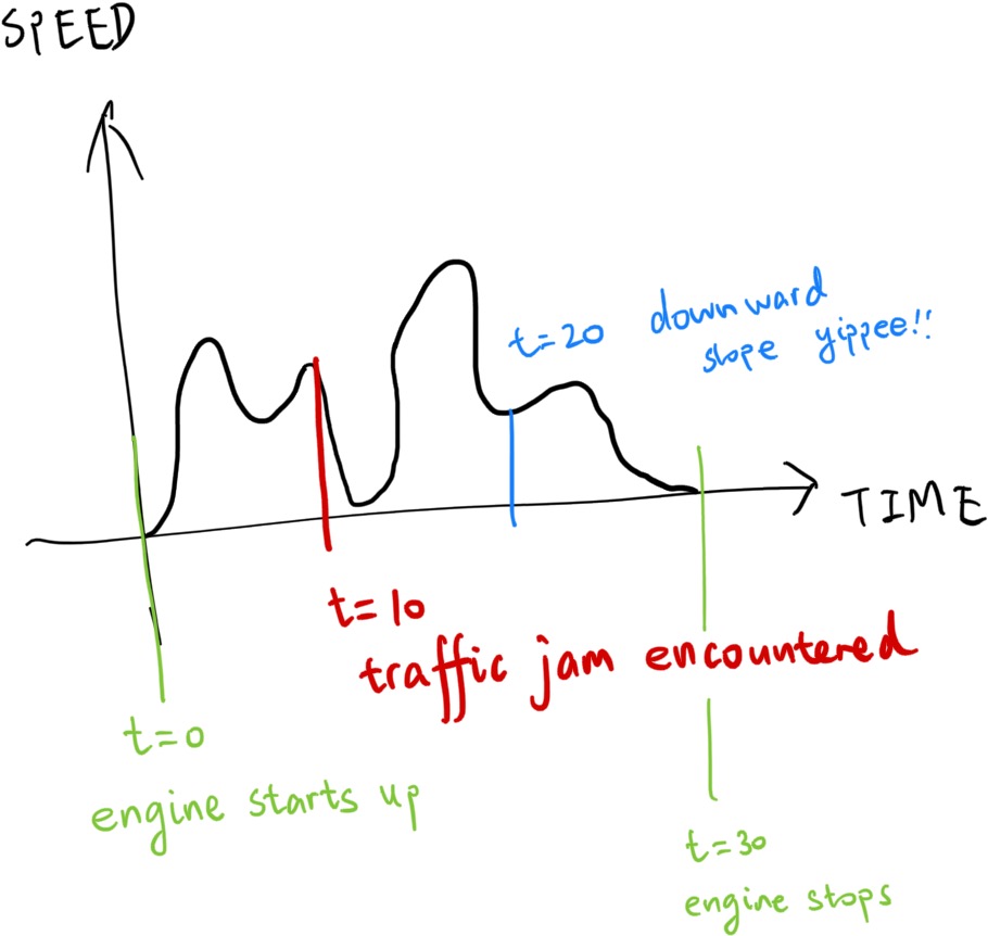
But humans are clever and they figured out another way. If we have a speed query function \(v\), and the speed query function can return the car’s speed at any given second, then we can estimate the total distance traveled by integrating the speed query function over the time the car spent in traveling.

\[s = \int_{t=0}^{T} v(t) dt\]

Now the speed query function is actually called the speed distribution. The underlying principle is the same: we are still doing the \(s = v t\), but now, we are doing it on a microscopic scale. We calculate a lot of mini-distances \(ds = v(t) dt\), and then sum them up together, like SUM(A1:A∞) in Microsoft Excel.

The speed represents a better granularity version of distance, because with the speed distribution in hand, we can calculate how far the car has traveled given any time intervals. With this completely unrelated stuff out of the way, let’s get started on radiant energy.

Radiant Energy

How to know how bright something is? The energy of a single photon is

\[Q = \frac{h c}{\lambda},\]

in which h stands for Planck’s constant, c stands for the speed of light, and \(\lambda\) stands for the wavelength of the photon (representing color).

Every photon carries energy, when a photon hits a something, the energy is either absorbed or reflected.

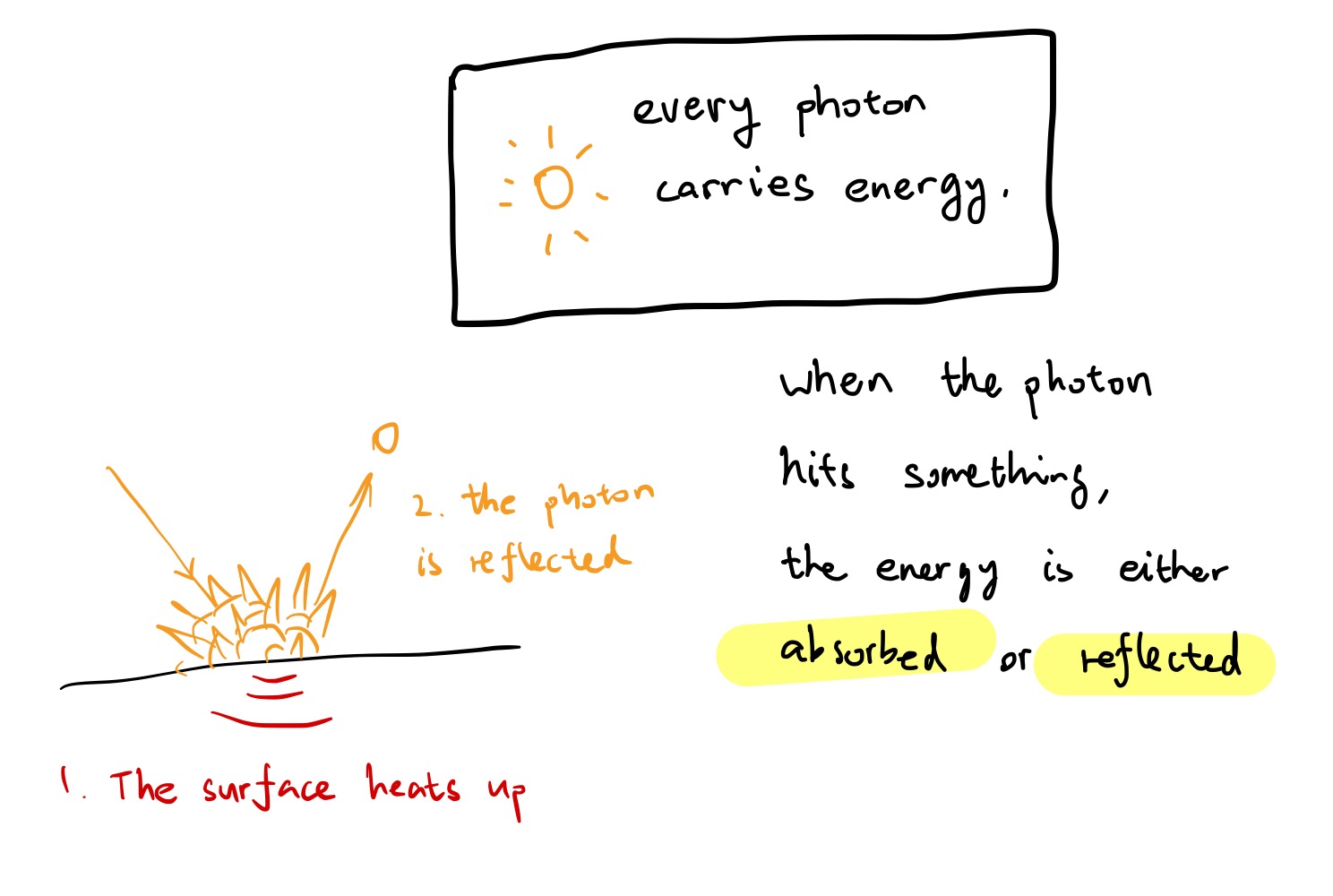
Imagine we have a light sensor. The radiant energy of the sensor is the amount of energy the sensor received over a period of time, and its unit is joules (J).

Radiant Flux

But radiant energy is too coarse a unit. Sun rises and sets, lights on and off, but the camera only captures one instant. We need something finer-grained to represent that, and so now we have radiant flux. The radiant flux measures the radiant energy per time, or joules per second (that’s watts!) of a given area. That’s

\[\Phi = \frac{dQ}{dt}\]

Recall the relation of speed and distance above. \(dQ\) in this context is equivalent to the mini-distance - we can get the radiant energy back if a radiant flux distribution is available.

Irradiance

If we are to determine, say, the color of the statue. While the radiant flux represents the radiant energy per time, it measures it for the whole given area. Just like the car’s speed is different at different points in time, the statue will have self occlusion parts and intricate details at different points of location, while missing in the others, causing a difference of mini-radiant flux. So, we need something finer-grained still. And that something is irradiance. Irradiance represents the radiant flux per area, or watts per square meter.

\[E(p) = \frac{d\Phi(p)}{dA}\]

Since \(dA\) is infinitesimal, we can say that it converges to a point. So an irradiance distribution can represent light information up to the granularity of one small point in a differential time. Just like integrating radiant flux over time results in radiant energy, integrating irradiance over the whole surface area yields us the radiant flux.

Radiant Intensity

Another way to add granularity to radiant flux is by breaking it up per solid angle instead of per area. This is especially useful for illuminants such as point lights, environment light maps, and so on, where the light intensity values are projected onto a sphere. (video from CMU15-462/662)

The unit of radiant intensity is watts per steradian. If you are unsure what steradian and solid angle is, I recommend checking out this slide from CMU15-462/662. As a differential solid angle is also infinitesimal, it converges to a direction.

\[I(\omega) = \frac{d\Phi(\omega)}{d\omega}.\]

The Inverse Square Law

Let’s list an example. Given the radiant intensity distribution of a point light, how do we get the irradiance of point p on a surface? We can basically just plug things in at this point.

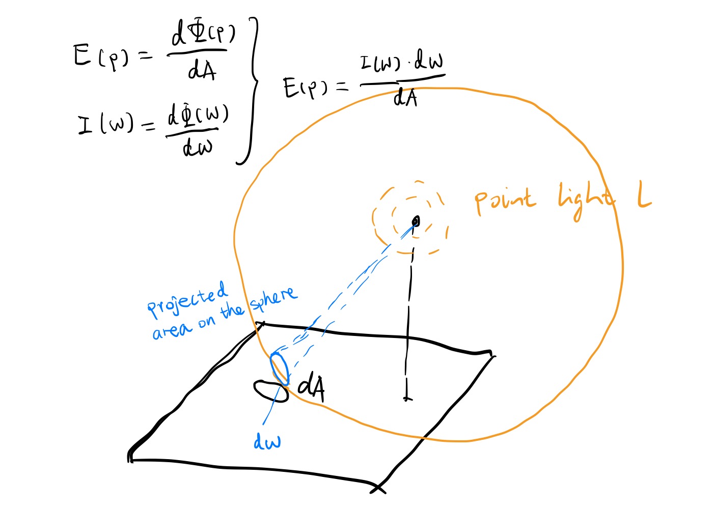
As solid angle and projected spherical area can be transferred between

\[\Omega = \frac{A_S}{r^2},\]

And the projected spherical area \(A_S\) is also a projection of A to sphere l, therefore,

\[A_S = A \cos \theta,\]

\(\theta\) being the angle between surface normal and incoming light direction. We can then plug this in the steradian equation and plug that in the irradiance equation, yielding

\[E(p) = \frac{I(\omega) \cos \theta}{r^2}.\]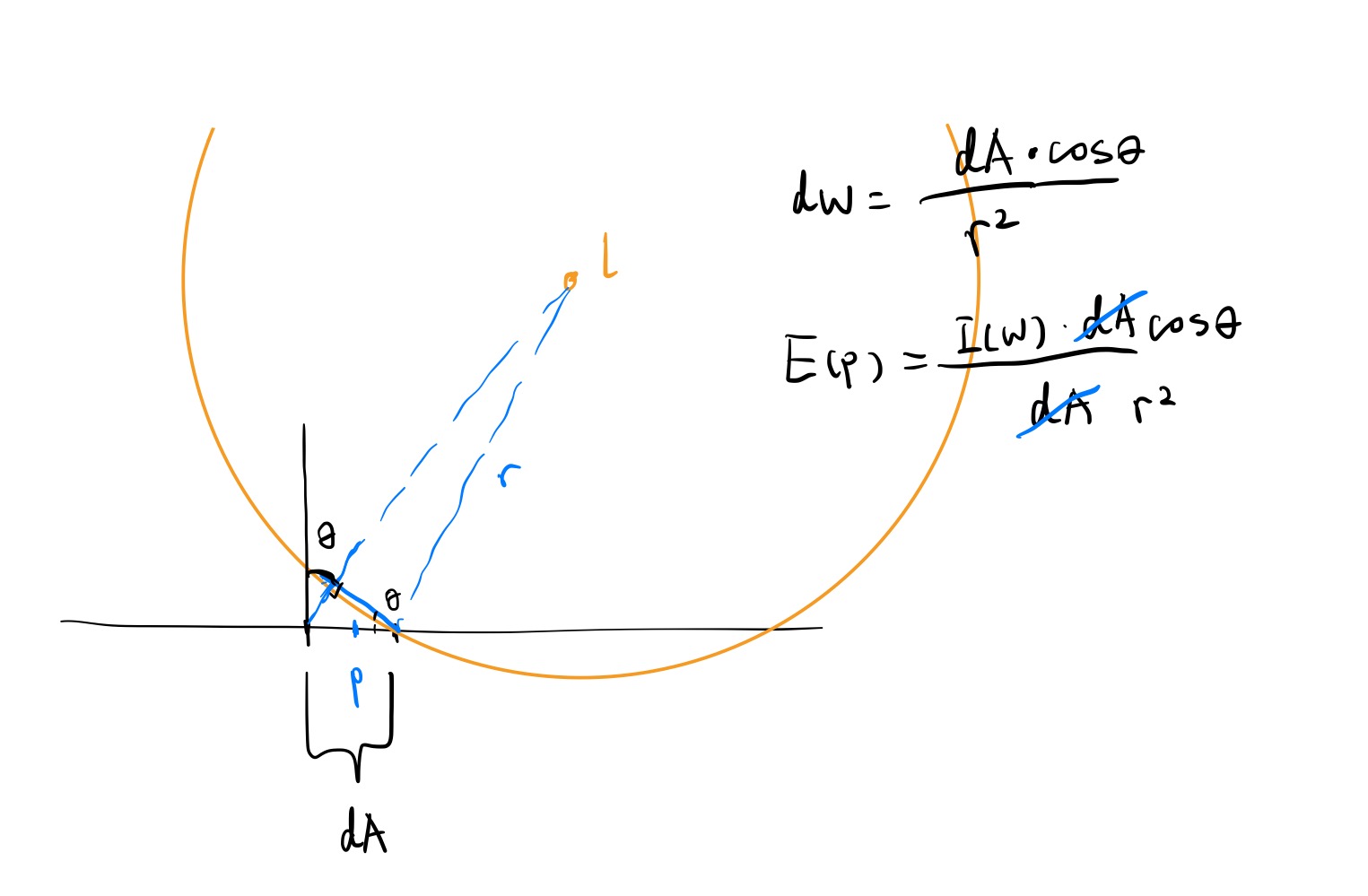

As we can see, the irradiance of a surface under a point light 1. gets smaller when \(\theta\) gets bigger, and 2. falls off quick as the light is farther and farther away. This is called the “inverse-square law” and is the typical light behavior in the real world.

Radiance

So, if we observe a surface patch and want to measure its brightness, do we measure its irradiance? Wrong. We obviously can’t see the reflected photons that’s not coming to our eyes. In other words, we are only interested in the irradiance fraction that is going towards the direction of the camera sensor. This requires us to break down irradiance even further. And here comes radiance, which is the solid angle density of irradiance.

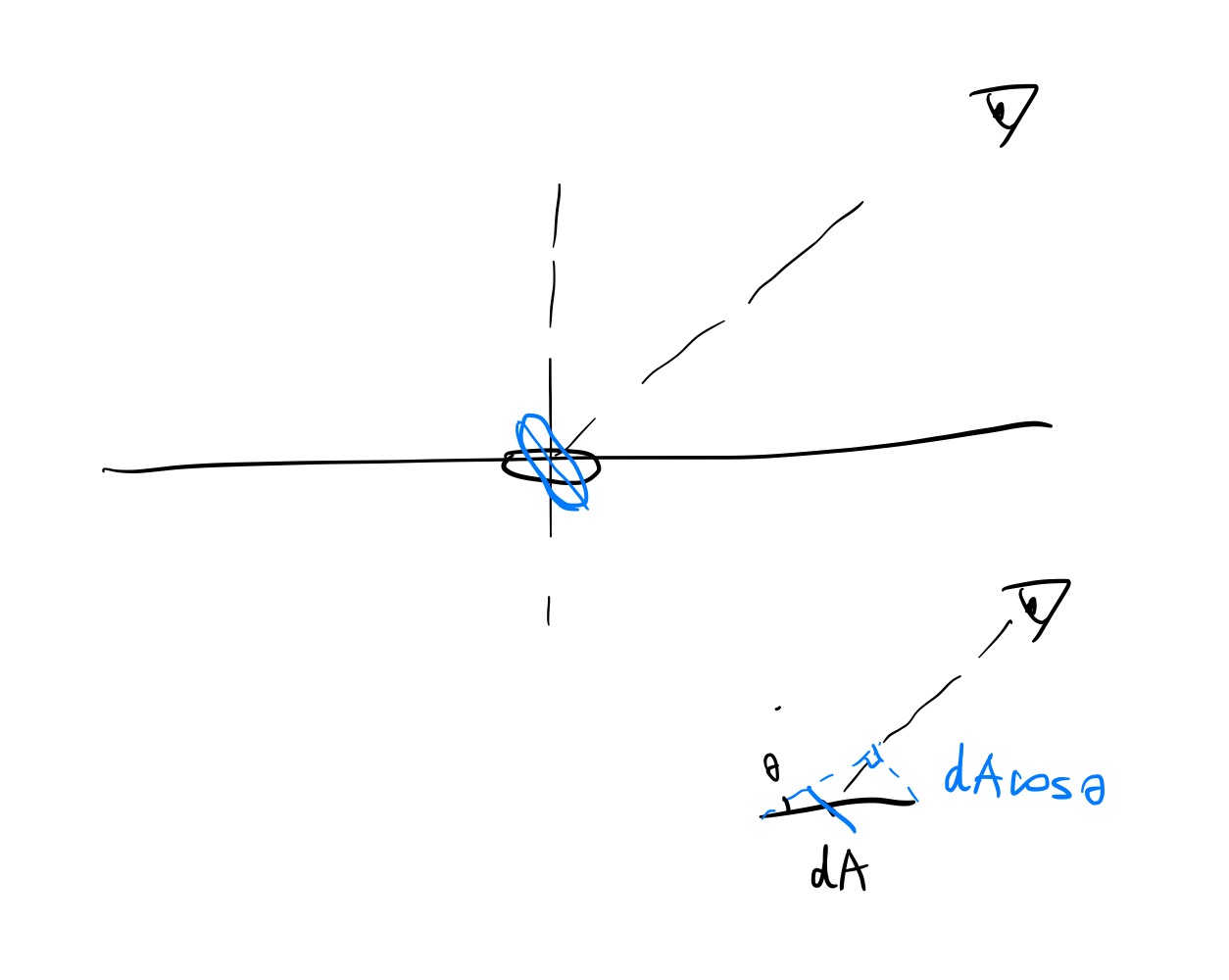
\[L(p, \omega) = \frac{dE_\omega(p)}{d\omega}\]

The surface area in the context of radiance is not orienting towards the surface itself, but rather, the viewing direction. So we have to correct that by adding a cosine term. The radiance therefore becomes

\[L(p, \omega) = \frac{d\Phi^2_\omega(p)}{d\omega \cos \theta dA},\]

or, in other words, radiant flux per solid angle per projected area.

Surface Irradiance from Radiance

The irradiance at point p can be reverse-calculated by using the above formula.

\[\begin{aligned} L(p, \omega) &= \frac{d\Phi^2_\omega(p)}{d\omega \cos \theta dA} \\ &= \frac{dE_\omega(p)}{d\omega \cos \theta} \end{aligned}\] \[E(p) = \int_\Omega L(p, \omega) \cos \theta d\omega\]

Huh, it’s starting to look kind of suspicious… Like I’ve seen it somewhere before. The equation states that the irradiance at point p is the hemispherical integral of all the outgoing radiance. Let’s denote outgoing radiance as \(L_o\) instead of L. Because why not.

\[E(p) = \int_\Omega L_o(p, \omega_o) \cos \theta_o d\omega_o\]

If the surface reflects everything, then the sum of incoming radiance should be equal to outgoing radiance. Also, sometimes the surface will be self-illuminating, so we need to count that in as well.

\[E(p) = E_e(p) + \int_\Omega L_i(p, \omega_i) \cos \theta_i d\omega_i\]

You know, this thing is quite close to what a camera captures. If instead of E(p), we get the outgoing radiance for a specific direction instead, we can get a recursive radiance-calculating equation, which states that the radiance at point p with the outgoing direction \(\omega_o\) is equal to the sum of the emitted radiance at point p and the integral of the incoming radiance over a hemisphere. Waaaait a minute…

The Rendering Equation

That’s the rendering equation, which states that the radiance at point p with the outgoing direction \(\omega_o\) is equal to the sum of the emitted radiance at point p and the integral of the incoming radiance over a hemisphere!

\[L_o(p, \omega_o) = L_e(p, \omega_o) + \int_\Omega f(p, \omega_o, \omega_i) L_i(p, \omega_i) \cos \theta_i d\omega_i\]

Just like speed is distance broken down using time, the rendering equation is also the surface irradiance from radiance equation broken down using solid angles. We can see that by integrating it back to surface irradiance:

\[\begin{aligned} \int_\Omega L_o(p, \omega_o) \cos \theta_o d\omega_o &= \int_{\Omega} [L_e(p, \omega_o) + \int_\Omega f(p, \omega_o, \omega_i) L_i(p, \omega_i) \cos \theta_i d\omega_i \cos \theta_o] d\omega_o \\ E(p) &= E_e(p) + \int_{\Omega} \int_{\Omega} f(p, \omega_o, \omega_i) L_i(p, \omega_i) \cos \theta_i d\omega_i \cos \theta_o d\omega_o \end{aligned}\]

The \(f\) function is the BRDF (Bidirectional Reflection Distribution Function), and it describes the angle-dependent factor of a surface:

\[f(p, \omega_o, \omega_i) = \frac{dL_o(p, \omega_o)}{dE_{\omega_i}(p)}\]

Plugging this back into the rendering equation integration and we get

\[\begin{aligned} E(p) &= E_e(p) + \int_{\Omega} \int_{\Omega} \frac{dL_o(p, \omega_o)}{dE_{\omega_i}(p)} L_i(p, \omega_i) \cos \theta_i d\omega_i \cos \theta_o d\omega_o \end{aligned}\]

Recall that for non-emitters, \(E = \int_\Omega L_i(p, \omega_i) \cos \theta_i d\omega_i\). That means \(dE_{\omega_i}(p) = L_i(p, \omega_i) \cos \theta_i d\omega_i\), effectively nuking a large part of the inner integration, and simplifying the equation to

\[\begin{aligned} E(p) &= E_e(p) + \int_{\Omega} L_o(p, \omega_o) \cos \theta_o d\omega_o. \end{aligned}\]

Now recall that if the surface is perfectly reflective, then the incoming radiance integration should be equal to the outgoing radiance integration. QED.

Conclusion

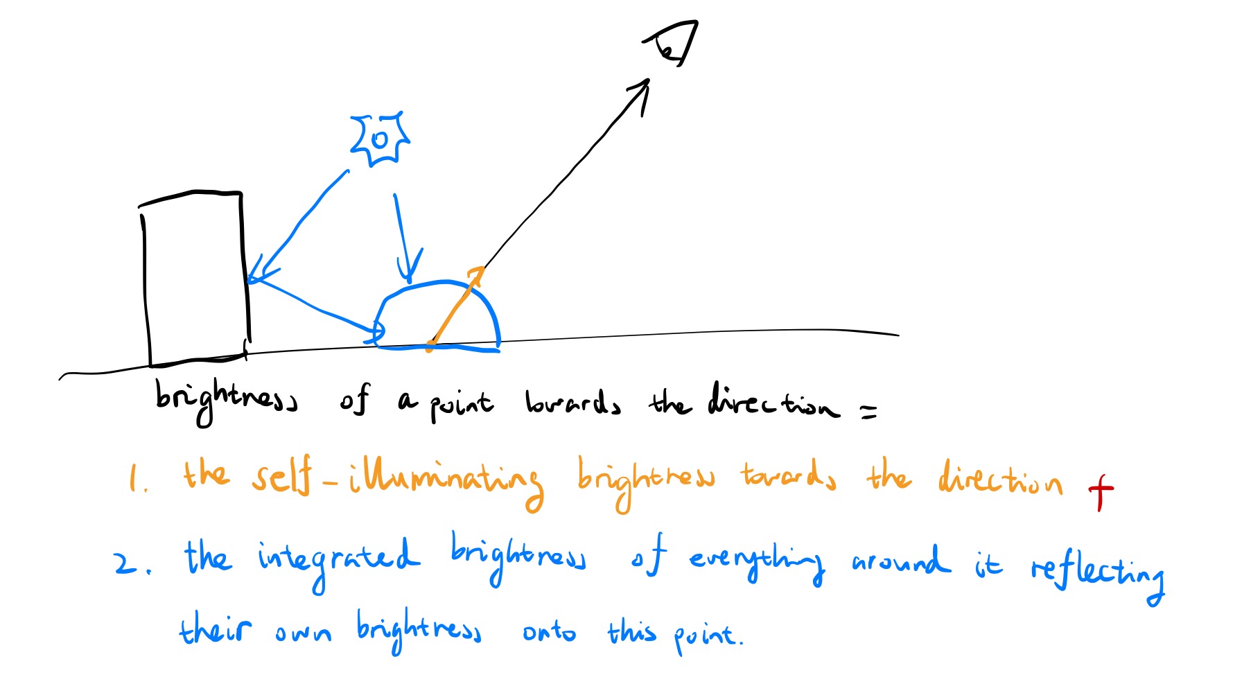
Whew, that’s quite a journey! But now you see, the rendering equation is just radiometry units broken into smaller and smaller pieces, each with more and more granularity. Sprinkle in a bit of mathematical magic, and you have yourself the fundamental equation for global illumination. Of course, if you want a more intuitive understanding, you can always remember that the rendering equation like this:

The brightness of a point towards a viewing direction is determined by the sum of the brightness of the self emitting part (if it is a lamp, sun, etc.) and the integrated brightness of everything around it reflecting their brightness onto this point.

Of course, that means we need to resolve the brightness coming from \(\omega_i\) first, using the very same rendering equation, and making it a recursive equation. And in the end, don’t forget about the BRDF!