We all know that Gaussian Splatting is the latest hit in novel view synthesis. In a massive nutshell, the 3D scene is recovered from multiple images via first passing through a COLMAP SfM, then things called “gaussians” are generated from the SfM points. These gaussians are then nudged around to fit the input images during the course of the training. If you are interested in the paper, definitely check out this video in conjunction with the paper. But we are not going over how the gaussians are trained today. Instead, we will be looking at this problem: when we’re given a trained gaussian splatting scene, how can we rasterize it?

At the end of the day, the “gaussians” the paper mentioned are just fancy ellipsoids. So the problem becomes, how do we render fancy ellipsoids fast (because boy there sure are a lot of ellipsoids), and can we do it without CUDA?

Note: if you are trying to follow & implement the same thing in this blog post, you can check out the modified SIBR_Viewers’s “ellipsoid” visualization method and use it as a reference, available on GitHub. The full source code of the rasterizer in this blog post is also available on GitHub.

The Scene File

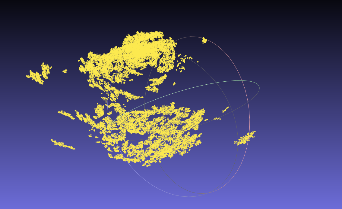
In any case, let’s first take a look at the trained scene. Gaussian Splatting is awesome because there’s no trained vendor lock-in; I have no idea if I used the right word. The trained scene is just one giant binary .PLY file, one which we can straight up open in MeshLab. Only we can’t really do that; we are only shown a bunch of points.

So how are we supposed to view it? Time to delve deeper and into SIBR_Viewers’s source code. Specifically, how RichPoint is defined.

Warning: this blog post will have tons of code segments. Sorry in advance. Especially you guys, mobile readers <3

template<int D>
struct RichPoint
{
    Pos pos;
    float n[3];
    SHs<D> shs;
    float opacity;
    Scale scale;
    Rot rot;
};

We learn that a RichPoint is just a vertex with extra properties:

1. Pos is a 3-dimensional vector.
2. SHs are a \((D + 1)^2\) array of 3-dimensional vectors used for spherical harmonics.
3. Scale is a 3-dimensional vector to denote scaling at the x, y, and z axis.
4. Rot is a 4-d vector to represent rotation in the form of a quaternion.

The PLY file is just densely-packed with these RichPoints. One extra thing to note though, the size of a RichPoint change depending on the spherical harmonics dimension, which is defined in your training parameters. But usually, when no training parameters are supplied, \(D = 3\). So let’s go ahead and just assume that - and then read the whole PLY model into memory.

// Short for "Gaussian Splatting Splats"
struct GSSplats
{
    bool valid; // Are the in-memory splats valid?
    int numSplats; // How many splats there are?
    std::vector<RichPoint> splats;
};

std::unique_ptr<GSSplats> GSPointCloud::loadFromSplatsPly(const std::string &path)
{
    std::unique_ptr<GSSplats> splats = std::make_unique<GSSplats>();
    splats->numSplats = 0;
    splats->valid = false;

    std::ifstream reader(path, std::ios::binary);
    if (!reader.good())
    {
        std::cerr << "Bad PLY reader: " << path << "?" << std::endl;
        return std::move(splats);
    }

    // Get the headers out of the way
    std::string buf;
    std::getline(reader, buf);
    std::getline(reader, buf);
    std::getline(reader, buf);
    std::stringstream ss(buf);
    std::string dummy;

    // Read the number of splats and resize the `splats` array
    ss >> dummy >> dummy >> splats->numSplats;
    splats->splats.resize(splats->numSplats);
    std::cout << "Loading " << splats->numSplats << " splats.." << std::endl;

    while (std::getline(reader, dummy))
    {
        if (dummy.compare("end_header") == 0)
        {
            break;
        }
    }

    // Read the whole thing into memory. "The lot", as they say.
    reader.read((char *) splats->splats.data(), splats->numSplats * sizeof(RichPoint));
    if (reader.eof())
    {
        std::cerr << "Reader is EOF?" << std::endl;
        splats->valid = false;
        return std::move(splats);
    }
    splats->valid = true;

    return std::move(splats);
}

The above code snippet will try to parse a trained PLY scene, and if it fails, or encountered EOF during reading, it returns an invalid GSSplat. Otherwise, it returns a valid PLY scene, with the points safely stored inside the splats vector.

What’s cool about this is the fact that by simply reading the scene, we already have enough information to visualize the scene (in the form of a point cloud). So let’s do that!

// ShaderBase::Ptr is just a shared_ptr<ShaderBase> with a .use() method
bool GSPointCloud::configureFromPly(const std::string &path, ShaderBase::Ptr shader)
{
    const auto splatPtr = loadFromSplatsPly(path);
    if (!splatPtr->valid)
    {
        return false;
    }

    _numVerts = splatPtr->numSplats;
    _shader = shader;

    // Initialize VAO and VBO
    glBindVertexArray(_vao);
    glBindBuffer(GL_ARRAY_BUFFER, _vbo);
    glBufferData(GL_ARRAY_BUFFER, sizeof(GSPC::RichPoint) * splatPtr->numSplats, splatPtr->splats.data(), GL_STATIC_DRAW);

    // #1: Set vertex attrib pointers
    constexpr int numFloats = 62;
    glEnableVertexAttribArray(0);
    glVertexAttribPointer(0, 3, GL_FLOAT, GL_FALSE, sizeof(float) * numFloats, nullptr);
    glEnableVertexAttribArray(1);
    glVertexAttribPointer(1, 3, GL_FLOAT, GL_FALSE, sizeof(float) * numFloats, (void *) (sizeof(float) * 6));

    // #2: Set the model matrix
    _model = glm::scale(_model, glm::vec3(-1.0f, -1.0f, 1.0f));

    return true;
}

We set the vertex attrib pointers in #1. Why 62 though? Well, one RichPoint is comprised of 62 floats in grand total:

We set two vertex attrib pointers: one for vertex positions, and the other for vertex colors. For the vertex color one, we simply use the first band of the spherical harmonics.

Then, in #2, we set the model matrix by flipping around the scene in Y axis and Z axis. For some weird reason, the scene is totally inverted - I am unsure as to why, but I guess it’s due to right hand/left hand shenanigans. Anyway, we need to correct that by setting the model matrix. Or, alternatively, you can also correct that by changing your camera’s arbitrary up as (0, -1, 0), which we will later do (and explain why). For now, setting the model matrix should suffice.

Next up, we implement our (very simple) vertex shader:

#version 430 core

layout (location = 0) in vec3 aPos;
layout (location = 1) in vec3 aSH;

// ... uniform MVP matrices

out vec3 color;

void main() {
    gl_Position = perspective * view * model * vec4(aPos, 1.0);
    color = aSH * 0.28 + vec3(0.5, 0.5, 0.5);
}

And fragment shader:

#version 430 core

in vec3 color;
out vec4 outColor;

void main() {
    outColor = vec4(color, 1.0);
}

And BAM! We have our point cloud, ladies and gentlemen.

Vertex Preprocessing

Obviously we can’t just stop at point clouds. Our target is to render the splats, after all. However, we have already half-succeeded since splats are just points enlarged to various forms (“gaussians” in our case). We can’t directly use the RichPoints though, not yet; we have to preprocess them.

The preprocessing involves:

1. Exponentiate scales;
2. Normalize quaternions;
3. And activate opacities (by passing them through a sigmoid function).

While we’re doing that, let’s transform the input data from a densely packed array of structures (AoS) into structure of arrays (SoA) as well. This is required since rendering splats are not as trivial as rendering points and will require new OpenGL functionalities.

std::vector<glm::vec4> positions;
std::vector<glm::vec4> scales;
std::vector<glm::vec4> colors;
std::vector<glm::vec4> quaternions;
std::vector<float> alphas;

positions.resize(splatPtr->numSplats);
// ... other resizes

for (int i = 0; i < splatPtr->splats.size(); i++)
{
    const glm::vec3 &pos = splatPtr->splats[i].position;
    positions[i] = glm::vec4(pos.x, pos.y, pos.z, 1.0f);

    const glm::vec3 &scale = splatPtr->splats[i].scale;
    scales[i] = glm::vec4(exp(scale.x), exp(scale.y), exp(scale.z), 1.0f);

    const SHs<3> &shs = splatPtr->splats[i].shs;
    glm::vec4 color = glm::vec4(shs.shs[0], shs.shs[1], shs.shs[2], 1.0f);
    colors[i] = color;

    quaternions[i] = glm::normalize(splatPtr->splats[i].rotation);

    alphas[i] = sigmoid(splatPtr->splats[i].opacity);
}

Rendering Splats

Our next problem is splat rendering. Again, recall that the “gaussians” are just fancy ellipsoids - so now, we have to render them. But how to rasterize one, really? OpenGL doesn’t really support the rendering of ellipsoids. Well, you’re in so much luck, because I just wrote a blog post on how to render them - enter Rendering a Perfect Sphere in OpenGL, then an Ellipsoid. Please go ahead and read that first!

Alright, have you read that? If you haven’t, I will make a short summary for you: the core idea is to first render the ellipsoid’s bounding box, then discard fragments during the fragment processing pass by checking if the camera ray hits the inner ellipsoid or not. One thing to add here is the fact that we are not just rendering one ellipsoid. Rather, we are rendering tens of thousands of them. This calls for the first technique we’ll have to use, and that is instancing.

1. Instance Render Cubes

We first create our cube VAO:

bool GSEllipsoids::configureFromPly(const std::string &path, ShaderBase::Ptr shader)
{
    const auto splatPtr = loadFromSplatsPly(path);
    if (!splatPtr)
    {
        return false;
    }
    _numInstances = splatPtr->numSplats;
    _numVerts = 36;

    glBindVertexArray(_vao);
    glBindBuffer(GL_ARRAY_BUFFER, _vbo);

    glBufferData(GL_ARRAY_BUFFER, sizeof(cube), cube, GL_STATIC_DRAW);
    glEnableVertexAttribArray(0);
    glVertexAttribPointer(0, 3, GL_FLOAT, GL_FALSE, sizeof(float) * 3, nullptr);

    return true;
}

The static cube variable is defined here. During rendering, we instance render the splat number of cubes:

_shader->use();
// ... uniforms

glBindVertexArray(_vao);
glDrawArraysInstanced(GL_TRIANGLES, 0, _numVerts, _numInstances);

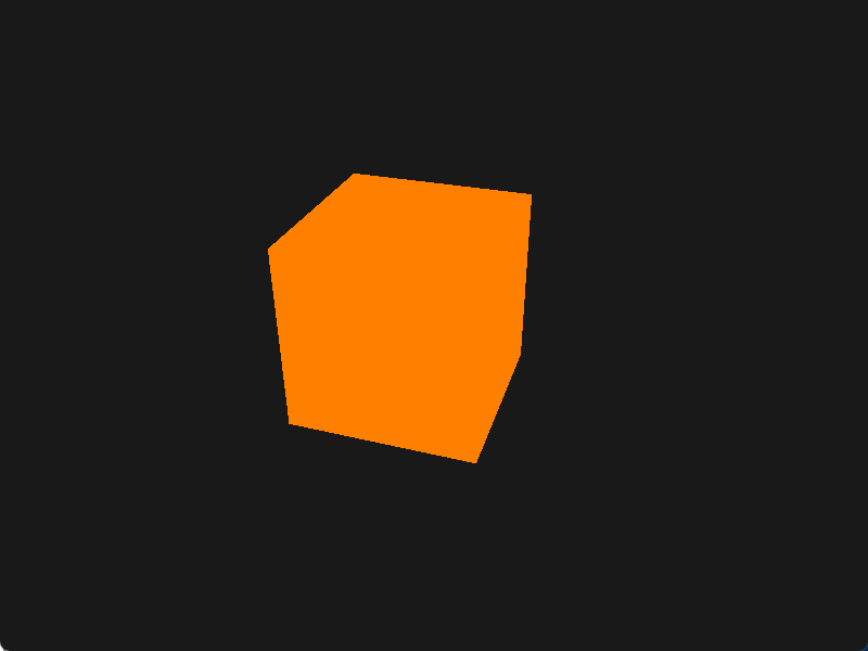
Now we have tens of thousands of cubes in one place. Cool! It is also unbelievably laggy.

2. Transform the Cubes

Next, we need to put the cubes into their proper places - as the cubes are the bounding boxes of the splats, the cube center should equal exactly to the center of the splats, as is the scales and rotations. How can we access these things in our shaders though? They are not available as vertex attributes; we only have the vertices of the cube for that. Or, we can try using Uniform Buffer Objects (UBO), but that falls short due to the large amount of data.

That, and the UBO requires a predetermined size before rendering, making using UBO unrealisitic. So how can we pass them into the shader? Time to bust out the big gun: Shader Storage Buffer Object (SSBO)! SSBOs are very much like UBOs, but without any of its shortcomings, and is generally just better. Their differences are:

1. SSBOs can be much, much larger. According to Khronos, UBOs can be to 16KB, but is implementation specific. In comparison, the spec guarantees SSBOs can be up to 128MB; most implementations can let you just use the whole GPU memory.
2. SSBOs are writable. In shader!
3. SSBOs can have variable storage. No more fixed size preallocation!
4. SSBOs are likely slower than UBOs.

Time to allocate 5 SSBOs, for positions, scales, colors, quaternions, and alphas, respectively. We can implement a template function capable of creating SSBOs of different atomic types, and it’s really simple:

template<typename T>
GLuint generatePointsSSBO(const std::vector<T> &points)
{
    GLuint ret = GL_NONE;
    glCreateBuffers(1, &ret);
    glNamedBufferStorage(ret, sizeof(T) * points.size(), points.data(), GL_MAP_READ_BIT);

    return ret;
}

Then we create SSBOs using

_positionSSBO = generatePointsSSBO(positions);
_scaleSSBO = generatePointsSSBO(scales);
_colorSSBO = generatePointsSSBO(colors);
_quatSSBO = generatePointsSSBO(quaternions);
_alphaSSBO = generatePointsSSBO(alphas);

And we’re good to go. Just don’t forget to delete them when the program exists via glDeleteBuffers. Pass the SSBOs into the shaders using glBindBufferBase:

_shader->use();
// ... uniforms

glBindBufferBase(GL_SHADER_STORAGE_BUFFER, 0, _positionSSBO);
glBindBufferBase(GL_SHADER_STORAGE_BUFFER, 1, _scaleSSBO);
glBindBufferBase(GL_SHADER_STORAGE_BUFFER, 2, _colorSSBO);
glBindBufferBase(GL_SHADER_STORAGE_BUFFER, 3, _quatSSBO);
glBindBufferBase(GL_SHADER_STORAGE_BUFFER, 4, _alphaSSBO);

glBindVertexArray(_vao);
glDrawArraysInstanced(GL_TRIANGLES, 0, _numVerts, _numInstances);

Next up, set the buffers to their respective binding points in our vertex shader. We can now access them by using positions[gl_InstanceID] etc.

layout (std430, binding = 0) buffer splatPosition {
    vec4 positions[];
};
layout (std430, binding = 1) buffer splatScale {
    vec4 scales[];
};
layout (std430, binding = 2) buffer splatColor {
    vec4 colors[];
};
layout (std430, binding = 3) buffer splatQuat {
    vec4 quats[];
};
layout (std430, binding = 4) buffer splatAlpha {
    float alphas[];
};

With all these in our hands, we can now transform the input vertices to their correct position.

// layout (std430, ...

out vec3 position;
out vec3 ellipsoidCenter;
out vec3 ellipsoidScale;
out mat3 ellipsoidRot;
out float ellipsoidAlpha;

void main() {
    // #1: scale the input vertices
    vec3 scale = vec3(scales[gl_InstanceID]);
    vec3 scaled = scale * aPos;

    // #2: transform the quaternions into rotation matrices
    mat3 rot = quatToMat(quats[gl_InstanceID]);
    vec3 rotated = rot * scaled;

    // #3: translate the vertices
    vec3 posOffset = rotated + vec3(positions[gl_InstanceID]);
    vec4 mPos = vec4(posOffset, 1.0);

    // #4: pass the ellipsoid parameters to the fragment shader
    position = vec3(mPos);
    ellipsoidCenter = vec3(positions[gl_InstanceID]);
    ellipsoidScale = scale;
    ellipsoidRot = rot;
    ellipsoidAlpha = alphas[gl_InstanceID];

    gl_Position = perspective * view * model * mPos;
    color = vec3(colors[gl_InstanceID]) * 0.28 + vec3(0.5, 0.5, 0.5);
}

We will need to first scale the vertices, then rotate them, then finally translate them, as shown in #1, #2, and #3. Imagine if we are transforming a sphere. If we rotate the sphere first then scale it, it wouldn’t make much sense: rotating a sphere is completely meaningless as spheres are rotation invariant. So we have to transform them in this order. In #2, we transform the quaternions into rotation matrices. Here I just Googled & used the quaternion-rotation matrix translation function from Automatic Addison; if you are interested and want to learn more about quaternions, do check out Visualizing Quaternions by Ben Eater and 3Blue1Brown.

mat3 quatToMat(vec4 q) {
    return mat3(2.0 * (q.x * q.x + q.y * q.y) - 1.0, 2.0 * (q.y * q.z + q.x * q.w), 2.0 * (q.y * q.w - q.x * q.z), // 1st column
                2.0 * (q.y * q.z - q.x * q.w), 2.0 * (q.x * q.x + q.z * q.z) - 1.0, 2.0 * (q.z * q.w + q.x * q.y), // 2nd column
                2.0 * (q.y * q.w + q.x * q.z), 2.0 * (q.z * q.w - q.x * q.y), 2.0 * (q.x * q.x + q.w * q.w) - 1.0); // last column
}

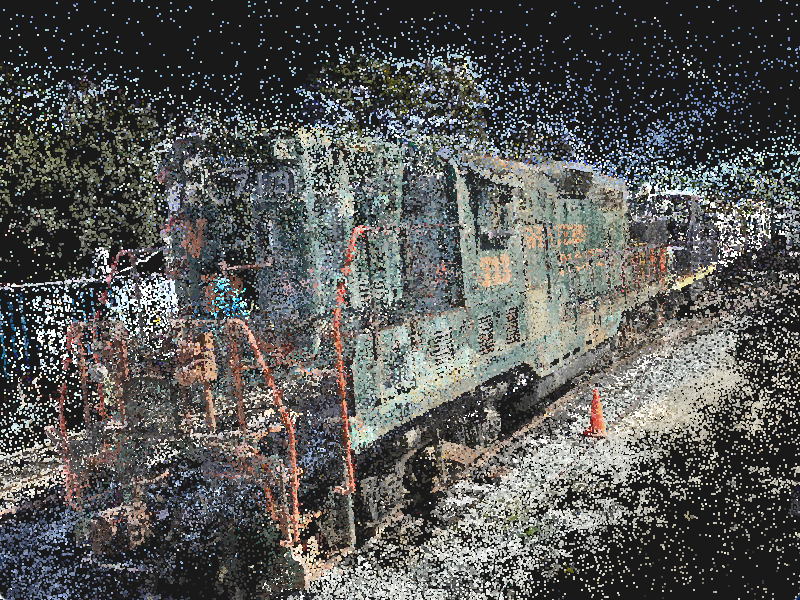
In #4, we pass all the ellipsoid parameters into the fragment shader to perform sphere tracing later; let’s not do that now though. What happens if we try to visualize the result now? It’s quite interesting, as it is already very close to the actual scene. We can even walk around and take a look.

Warning: large video! (13.2MB)

3. Turn Cubes into Ellipsoids

The final step involves tracing rays into the screen and determining if any of them hits the ellipsoids within the bounding boxes. Again, give this blog post a read if you want to properly understand how. With all these information we have though, it is more than enough for us to render the ellipsoids.

in vec3 position;
in vec3 ellipsoidCenter;
in vec3 ellipsoidScale;
in float ellipsoidAlpha;
in mat3 ellipsoidRot;
in vec3 color;

uniform vec3 camPos;
// ... MVP uniforms

out vec4 outColor;

void main() {
    vec3 normal = vec3(0.0);

    // Check if we intersects with the sphere given the ellipsoid center, scale, and rotation.
    // Normal is an output variable; we can additionally obtain the normal once we know there is an intersection.
    vec3 intersection = sphereIntersect(ellipsoidCenter, camPos, position, normal);

    // Discard if there's no intersections
    if (intersection == vec3(0.0)) {
        discard;
    }

    vec3 rd = normalize(camPos - intersection);
    float align = max(dot(rd, normal), 0.1);

    vec4 newPos = perspective * view * model * vec4(intersection, 1.0);
    newPos /= newPos.w;
    gl_FragDepth = newPos.z;

    // Lightly shade it by making it darker around the scraping angles.
    outColor = vec4(align * color, 1.0);
}

The fragment depth is updated once an intersection is found. Since the world position of the shading point, which is on the box, is different to the world position of the inner ellipsoid, we have to reproject the position to NDC and set the depth appropriately. And if we can obtain the normal from the intersection check, might as well shade it a little bit to make it look exactly like the ellipsoids in SIBR_Viewers.

Warning: large video! (13.2MB)

This is also when we have to ditch the model matrix flip and change the camera to upside down instead. The sphere tracing have not accounted for the model matrix and will result in all sorts of janky ellipsoids.

4. Some Extra Modifications

The result is quite close but some places are still unsatisfactory. For example, there are a lot of noisy ellipsoids in the way during our visualization blocking most of the view. Fixing that is simple enough: those ellipsoids usually have a very low alpha value, so we can filter them out easily via a simple alpha threshold check.

void main() {
    if (ellipsoidAlpha < 0.3) {
        discard;
    }

    vec3 normal = vec3(0.0);
    vec3 intersection = sphereIntersect(...

This can greatly clean up the scene:

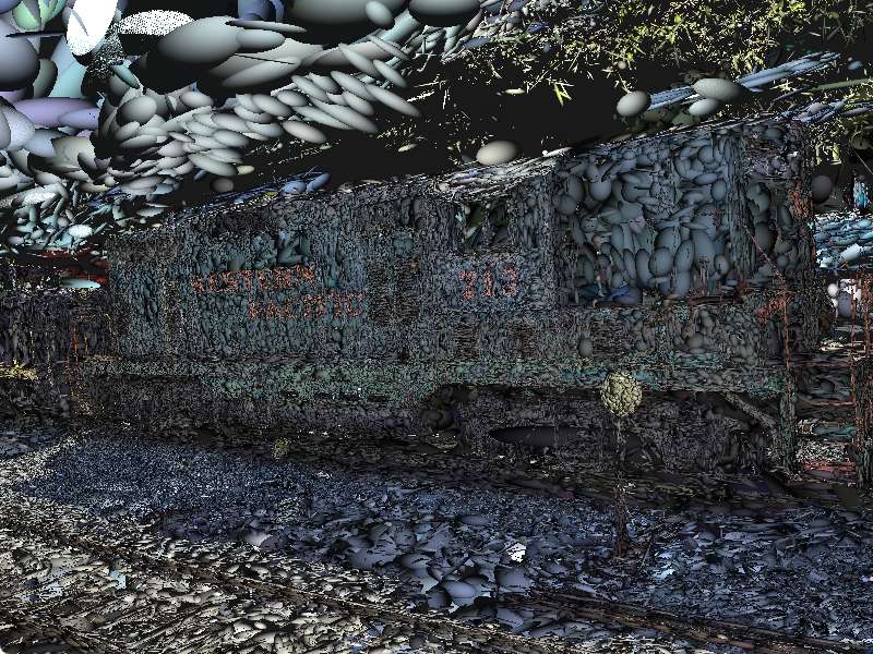
And finally, let’s scale the size of each ellipsoids by 2. I have no concrete idea why, but it is what SIBR_Viewers has done.

void main() {
    vec3 scale = vec3(scales[gl_InstanceID]) * 2.0;
    vec3 scaled = scale * aPos;
    mat3 rot = quatToMat(...

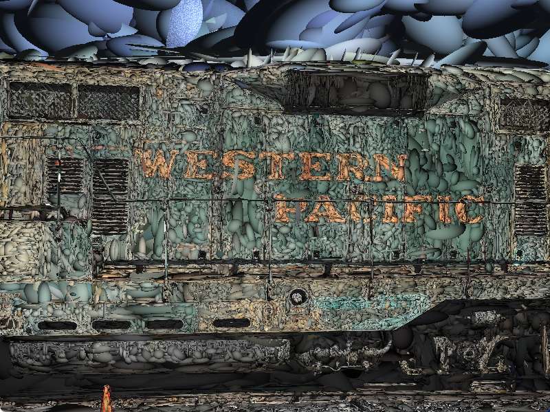
It has the benefit of making the text on the train much more prominent and easier to read (take a look at “Western Pacific”). Though, the frame rate drops greatly, probably due to the fact that we now need to trace more rays for each ellipsoid:

And that’s it!

Wait, what?!

Isn’t it supposed to look like this though?

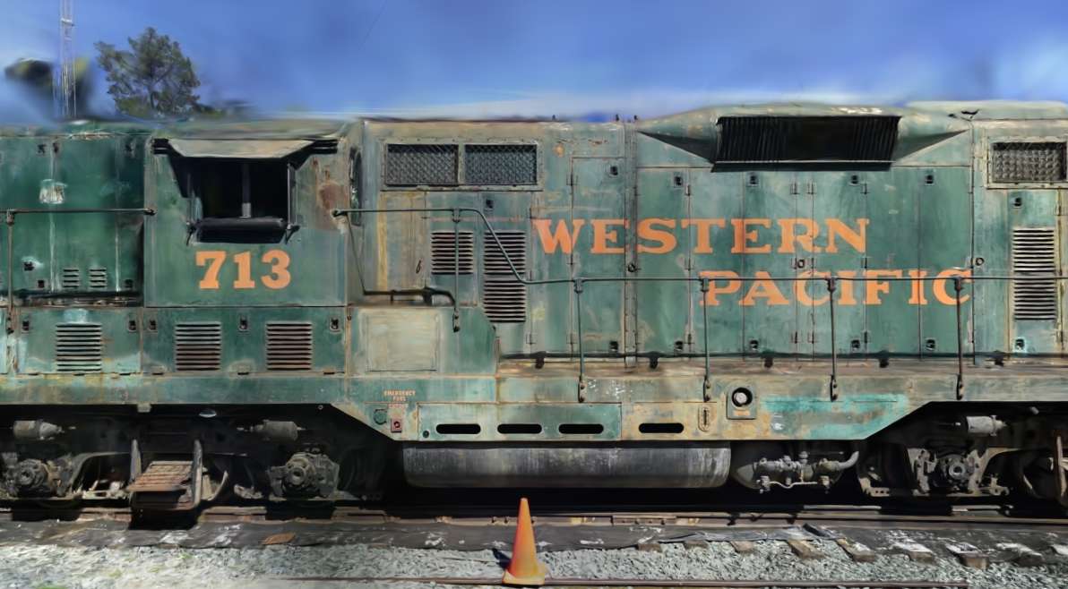
Yeah, but this render is done in CUDA. Though we have avoided CUDA throughout this blog post, and achieved… results, there is something that OpenGL can just not do. The most powerless one being alpha blending.

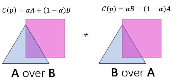
I have missed one key thing in the paragraphs above. “Gaussians” are not only ellipsoids; they are transparent ellipsoids, as seen in the alpha part of RichPoint. This means we have to perform alpha composition during the rendering of our gaussians. But alpha compositing is non-commutative; that is, A over B is not equal to B over A.

To perform alpha composition correctly, we have to render the furthest thing first, then composite it bit by bit until the closest. Putting into context of our gaussian splat rendering program, this means we need to sort the splats by depth relative to the camera every frame. Because the viewing camera is constantly on the move, we have to re-calculate it every frame, in case the order of splats change between frames. OpenGL alone is obviously not enough; not to mention that instanced rendering, the thing that makes us have more than 1 FPS in the first place, totally ignores the drawing order.

However, not all hope is lost. If we have some (very quick) method capable of sorting more than two hundred thousand splats by depth per-frame, we may just be onto something. After that, we can compute the real SH color in the fragment shader as well, by taking all 16 coefficients into consideration. Then maybe, just maybe, we can avoid using CUDA altogether. For now though, CUDA offers much better flexibility during splat rasterization, so it will have to do - and we’ll have another blog post on how to properly rasterize the gaussian splats in the unspecified future.

Again, if you are interested in the implementation of the rasterizer in this blog post, the full source code is available online on GitHub, so go and take a look. Until then, toodles!

Comments

A valid, non-empty username is required.

Comment